Continuing from the previous chapter, we have published three articles in the series of articles on Building a Powerful Crypto-Asset Portfolio Using Multi-Factor Models:Theoretical Basics、Data Preprocessing、Factor Validity Test。

The first three articles explain the theory of multi-factor strategy and the steps of single-factor testing respectively.

1. Reasons for factor correlation testing: multicollinearity

We screen out a batch of effective factors through single-factor testing, but the above factors cannot be directly entered into the database. The factors themselves can be divided into broad categories according to specific economic meanings. There is a strong correlation between factors of the same type. If they are directly entered into the database without correlation screening and multiple linear regression is performed to calculate the expected return rate based on different factors, there will be Multicollinearity problem. In econometrics, multicollinearity means that some or all explanatory variables in a regression model have a complete or accurate linear relationship (high correlation between variables).

Therefore, after the effective factors are screened out, it is first necessary to conduct a T test on the correlation of factors according to major categories. For factors with higher correlation, either discard factors with lower significance or perform factor synthesis.

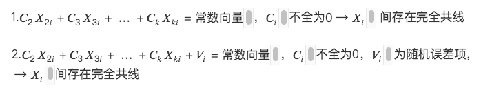
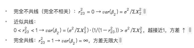
The mathematical explanation of multicollinearity is as follows:

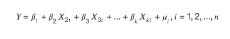
There will be two situations:

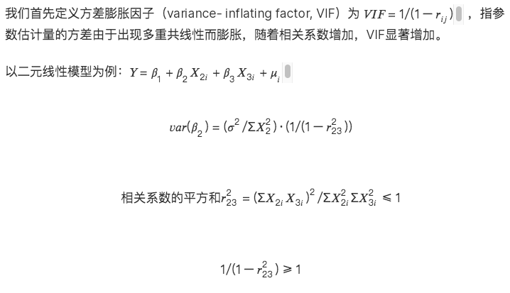
Consequences of multicollinearity:

1. Parameter estimators do not exist under perfect collinearity

2. OLS estimator is not valid under approximate collinearity

3. The economic significance of parameter estimators is unreasonable

4. The significance test of the variable (t test) loses significance

5. The prediction function of the model fails: the predicted return rate fitted by the multivariate linear model is extremely inaccurate, and the model fails.

2. Step 1: Correlation test of factors of the same type

Test the correlation between the newly calculated factors and the factors already in the database. Generally speaking, there are two types of data for correlation:

1. Calculate the correlation based on the factor values ​​of all tokens during the backtest period

2. Calculate the correlation based on the factor excess return values ​​of all tokens during the backtest period

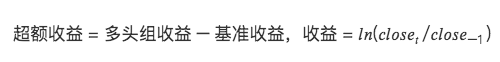
Each factor we seek has a certain contribution and explanatory power to the tokens return rate. The purpose of conducting correlation testing** is to find factors that have different explanations and contributions to strategy returns. The ultimate goal of the strategy is returns**. If two factors describe returns the same, it is meaningless even if the two factor values ​​are significantly different. Therefore, we did not want to find factors with large differences in factor values ​​themselves, but wanted to find factors with different factors describing returns, so we finally chose to use factor excess return values ​​to calculate correlations.

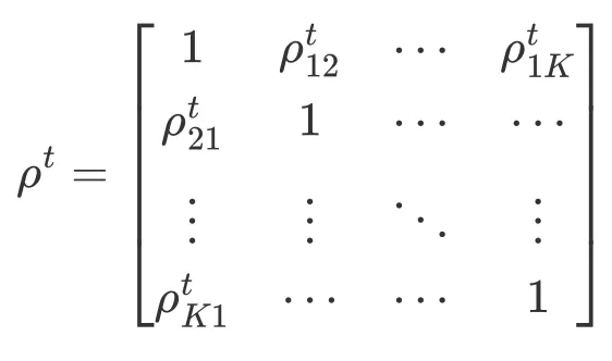
Our strategy is daily frequency, so we calculate the correlation coefficient matrix between factor excess returns based on the date of the backtest interval.

Programmatically solve for the top n factors with the highest correlation in the library:

def get_n_max_corr(self, factors, n= 1):
       factors_excess = self.get_excess_returns(factors)
       save_factor_excess = self.get_excess_return(self.factor_value, self.start_date, self.end_date)
       if len(factors_excess) < 1:
           return factor_excess, 1.0, None
       factors_excess[self.factor_name] = factor_excess['excess_return']
       factors_excess = pd.concat(factors_excess, axis= 1)
       factors_excess.columns = factors_excess.columns.levels[ 0 ]
       # get corr matrix
       factor_corr = factors_excess.corr()
       factor_corr_df = factor_corr.abs().loc[self.factor_name]
       max_corr_score = factor_corr_df.sort_values(ascending=False).iloc[ 1:].head(n)
       
       return save_factor_excess, factor_corr_df, max_corr_score

3. Step 2: Factor selection and factor synthesis

For factor sets with high correlation, there are two ways to deal with them:

(1) Factor selection

Based on the ICIR value, yield, turnover rate, and Sharpe ratio of the factor itself, the most effective factors in a certain dimension are selected to retain and other factors are deleted.

(2) Factor synthesis

Synthesize the factors in the factor set and retain as much effective information as possible on the cross-section

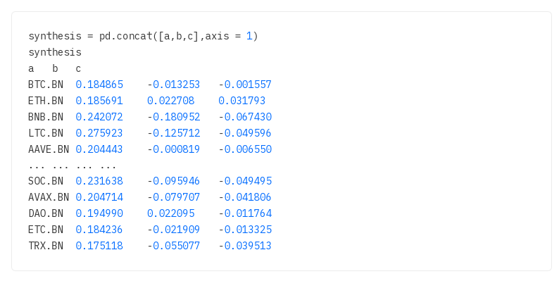
Assume that there are currently 3 factor matrices to be processed:

2.1 Equal weighting

The weight of each factor is equal (w= 1/number of factors), and the comprehensive factor = the sum of the values ​​of each factor is averaged.

Eg. Momentum factors, one-month rate of return, two-month rate of return, three-month rate of return, six-month rate of return, twelve-month rate of return. The factor loadings of these six factors each account for 1/6 of the weight. , synthesize new momentum factor loadings, and then perform normalization again.

synthesis 1 = synthesis.mean(axis= 1) # Find the mean by row

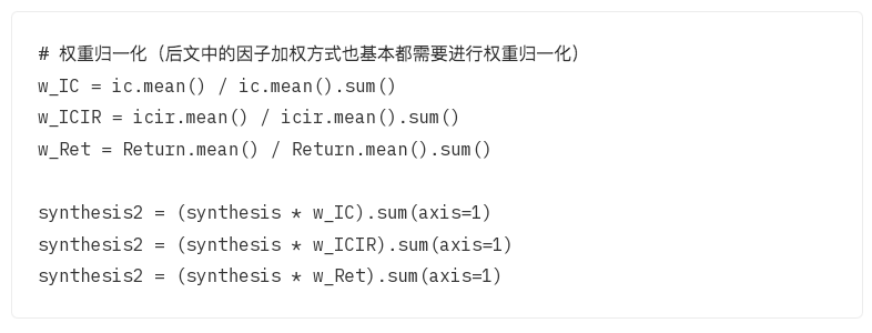
2.2 Historical IC weighting, historical ICIR, historical income weighting

Factors are weighted by their IC values ​​(ICIR values, historical return values) over the backtest period. There have been many periods in the past, and each period has an IC value, so their mean is used as the weight of the factor. It is common to use the mean (arithmetic mean) of the IC over the backtest period as the weight.

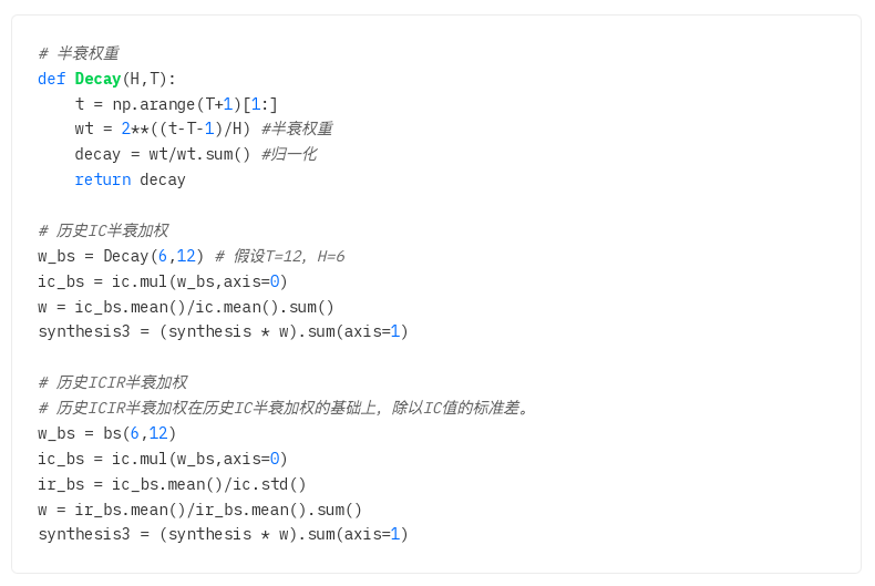
2.3 Historical IC half-life weighting, historical ICIR half-life weighting

2.1 and 2.2 both calculate the arithmetic mean, and each IC and ICIR in the backtest period have the same effect on the factor by default.

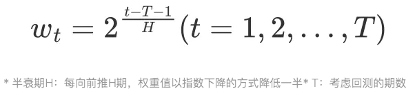
However, in reality, the impact of each period of the backtest period on the current period is not exactly the same, and there is a time attenuation. The closer the period is to the current period, the greater the impact, and the further away the impact is, the smaller it is. Based on this principle, before calculating the IC weight, first define a half-life weight. The closer to the current period, the larger the weight value, and the further away, the smaller the weight.

Mathematical derivation of half-life weight:

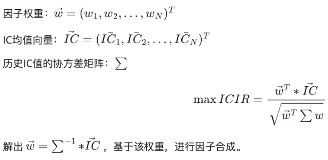
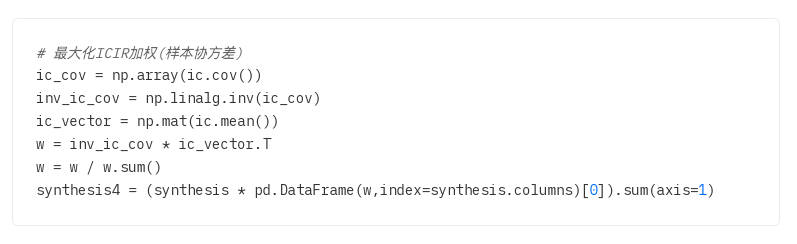
2.4 Maximize ICIR weighting

By solving the equation, calculate the optimal factor weight w to maximize the ICIR

Covariance matrix estimation problem: The covariance matrix is ​​used to measure the correlation between different assets. In statistics, the sample covariance matrix is ​​often used instead of the population covariance matrix. However, when the sample size is insufficient, the sample covariance matrix and the population covariance matrix will be very different. Therefore, someone proposed a compression estimation method. The principle is to minimize the mean square error between the estimated covariance matrix and the actual covariance matrix.

Way:

1. Sample covariance matrix

2. Ledoit-Wolf shrinkage: Introduce a shrinkage coefficient to mix the original covariance matrix with the identity matrix to reduce the impact of noise.

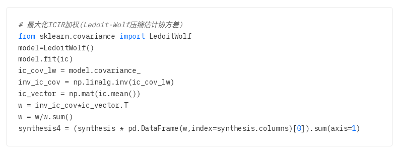
3. Oracle Approximate Shrinkage: An improvement over Ledoit-Wolf shrinkage, the goal is to more accurately estimate the true covariance matrix when the sample size is small by adjusting the covariance matrix. (The programming implementation is the same as Ledoit-Wolf shrinkage)

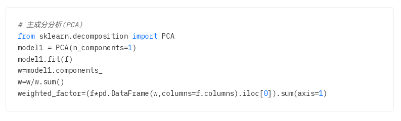
2.5 Principal component analysis PCA

Principal Component Analysis (PCA) is a statistical method used to reduce dimensionality and extract the main features of data. The goal is to map the original data to a new coordinate system through linear transformation to maximize the variance of the data in the new coordinate system.

Specifically, PCA first finds the principal components in the data, which is the direction with the largest variance in the data. It then finds the second principal component that is orthogonal (unrelated) to the first principal component and has the largest variance. This process is repeated until all principal components in the data are found.