Original text author: Fox Tech CEO Kang Shuiyue, Fox Tech Chief Scientist Meng Xuanji

Foreword: If cryptographers do not discover the connection between Tensor Product and polynomial values, it will be difficult for the polynomial commitment protocol Brakedown to appear, and it will be impossible to produce new ones such as Brakedown-based Orion and FOAKS. Fast algorithm.

In many zero-knowledge proof systems that rely on polynomial commitments, different commitment protocols are used. According to the evaluation of Justin Thaler of a16z in the article "Measuring SNARK performance: Frontends, backends, and the future" in August 2022, although Brakedown has a larger Proof Size, it is undoubtedly the fastest polynomial commitment protocol at present.

FRI, KZG, Bulletproof are more common polynomial commitment protocols, but speed is their bottleneck. Algorithms such as Plonky used by zkSync, Plonky 2 used by Polygon zkEVM, and Ultra-Plonk used by Scroll are all polynomial commitments based on KZG. Prover involves a large number of FFT calculations and MSM operations generating polynomials and commitments, both of which impose a large computational burden. Although MSM has the potential to run multi-threaded acceleration, it requires a lot of memory and is slow even under high parallelism, while large-scale FFT relies heavily on the frequent shuffling of data when the algorithm is running, making it difficult to load across computing clusters through distributed acceleration.

It is precisely because of the faster polynomial commitment protocol Brakedown that the complexity of such operations is greatly reduced.

FOAKS, or Fast Objective Argument of Knowledges, is a Brakedown-based zero-knowledge proof system framework proposed by Fox Tech. FOAKS further reduces FFT operation on the basis of Orion, and the goal is to eliminate FFT eventually. In addition, FOAKS also designed a new and very elegant proof recursion method to reduce the proof size. The advantage of the FOAKS framework is that it has a small proof size based on the realization of linear proof time, which is very suitable for zkRollup scenarios.

Below we will introduce the polynomial commitment protocol Brakedown used by FOAKS in detail.

In cryptography, the commitment (Commitment) protocol consists of the prover (Prover) committing to a certain secret value, generating a public commitment value, which has binding and hiding (Hiding), and then submits The verifier needs to open this promise and send the message to the verifier to verify the correspondence between the promise and the message. This makes commitment protocols and hash functions have a lot in common, but commitment protocols often rely on mathematical structures in the field of public key cryptography. The polynomial commitment (Polynomial Commitment) is a type of commitment scheme for polynomials, that is to say, the promised value is a polynomial. At the same time, the polynomial commitment protocol also includes an algorithm to obtain a value at a given point and give a proof, which makes the polynomial commitment protocol itself an important class of cryptographic protocols and the core part of many zero-knowledge proof systems.

In the latest research in the field of cryptography, due to the discovery of the connection between the tensor product (Tensor Product) and the value of the polynomial, a series of related polynomial commitment protocols were born, and Brakedown is one of the representative protocols. .

Before introducing the details of the Brakedown protocol in detail, some basics need to be understood. We need to understand the operations of Linear Code, Anti-collision Hash Function, Merkle Tree, Tensor Product and tensor product representation of polynomial values.

The first is the linear code (Linear Code). A linear code with message length k and code word length n is a linear subspace

C ∈ Fn, so that there is an injection from the message to the code word, called encoding, denoted as EC: Fk→C. Any linear combination of codewords is still a codeword. The distance between two codewords u and v is their Hamming distance, denoted as △(u, v).

The shortest distance is d=minu, v△(u, v). Such codes are denoted as [n, k, d] linear codes, and d /n represents the relative distance of the codes.

Followed by anti-collision hash function (Hash Function) and Merkle tree (Merkle Tree).

Use H: { 0, 1 } 2 λ → { 0, 1 } λ to represent a hash function. Merkle tree is a special data structure that can realize the promise of 2 d messages, generate a hash value h, and need d+ 1 hash value when opening any message.

A Merkle tree can be represented as a binary tree with depth d, where L message elements m1 , m2 ,..., ml correspond to the leaves of the tree respectively. Each internal node of the tree is hashed from its two child nodes. When opening a message mi, the path from mi to the root node needs to be disclosed.

image description

1. h←Merkle.Commit(m1 ,..., ml)

2. (mi,πi)←Merkle.Open(m, i)

3. { 0, 1 }←Merkle.Verify(πi, mi, h)

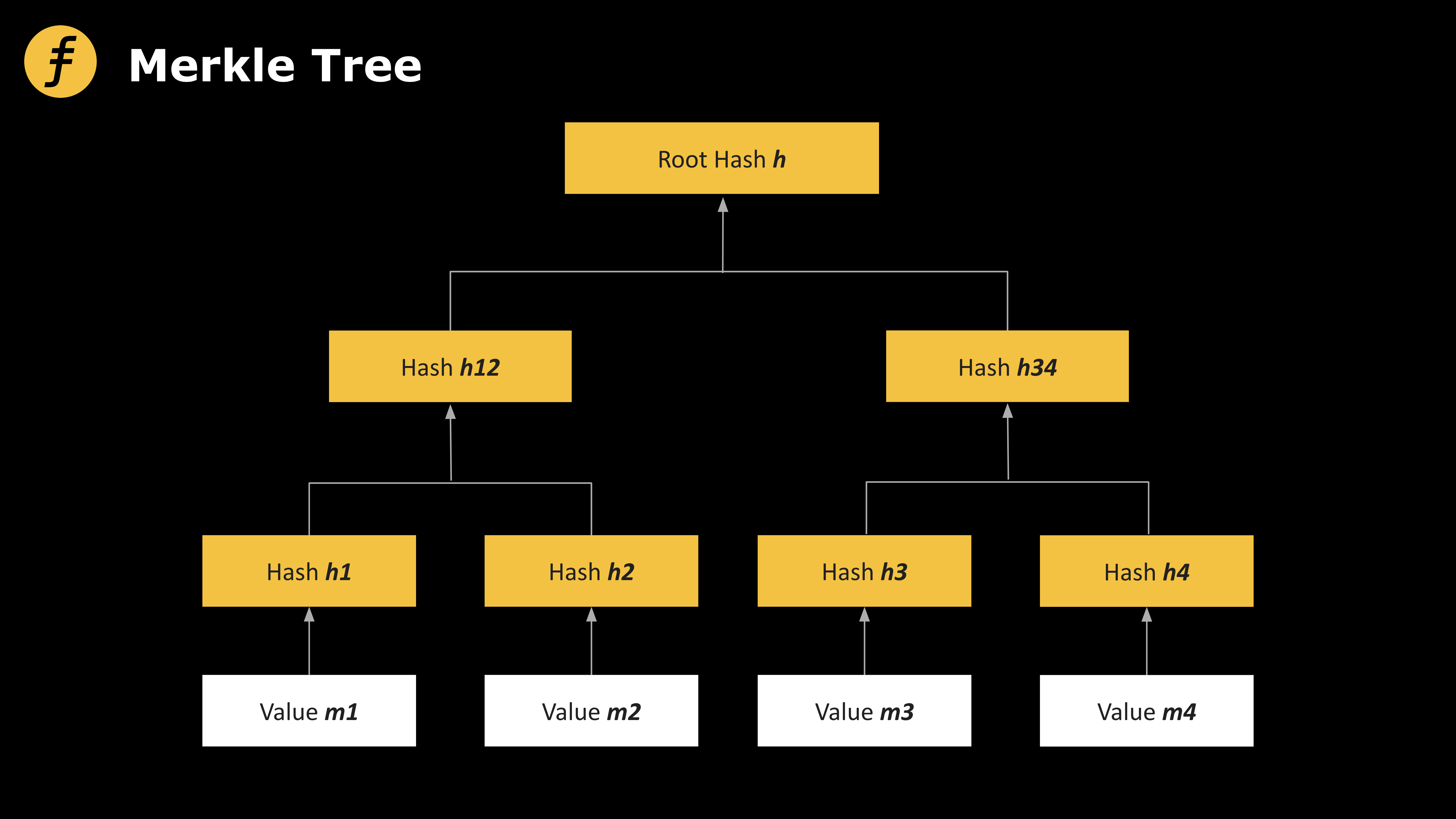
Figure 1: Merkle Tree

image description

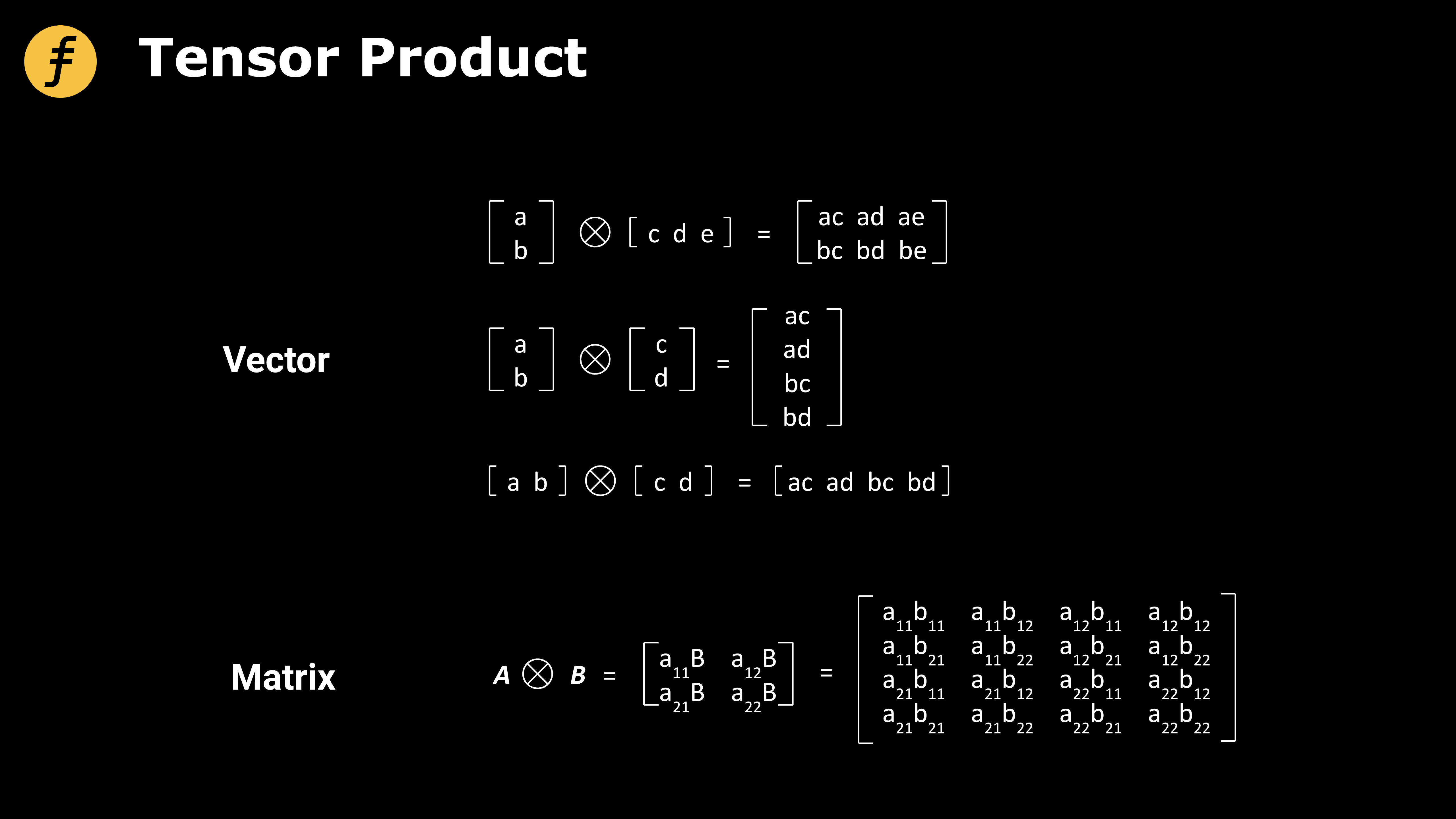
Figure 2: Tensor product operation of vectors and matrices

Next, we need to know the tensor product representation of the polynomial values.

As mentioned in [GLS+], the values ​​of polynomials can be expressed in the form of tensor products. Here we consider multilinear polynomial commitments.

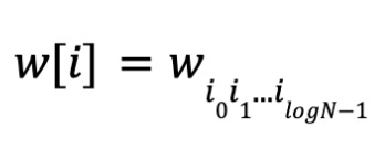
Specifically, given a polynomial, its values ​​in the vectors x0 , x1 ,..., xlogN-1 can be written as:

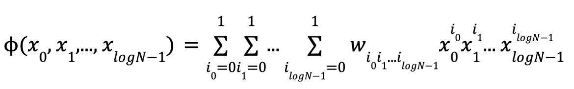
According to the definition of multilinearity, the degree of each variable is 0 or 1, so there are N monomials and coefficients, and logN variables. make

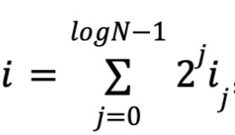
, where i0 i1 ...ilogN-1 is the binary representation of i. Let w denote the polynomial coefficients,

Similarly, define

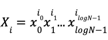
make

. So X=r0 ⊗r1.

Thus, polynomial values ​​can be expressed in the form of tensor products: ϕ(x0 , x1 ,..., xlogN-1 )=。

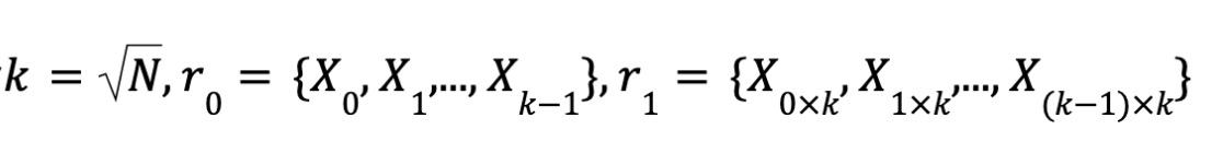
Finally, let's look at the Brakedown process used in FOAKS and Orion [XZS 22 ].

First, PC.Commit divides the polynomial coefficient w into a k×k matrix form, and codes it (refer to the linear code in "Preliminary Knowledge"), denoted as C2. Then make a commitment to each column C2 [:, i] of C2 to build a Merkle tree, and then build another Merkle tree for the root of the Merkle tree formed by each column as the final commitment.

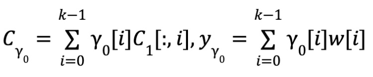
In the calculation of the value proof, two points need to be proved, one is proximity (Proximity), and the other is consistency (Consistency). Approximation ensures that the committed matrix is ​​indeed close enough to an encoded codeword. Consistency Guarantee y=。

Proximity testing: Proximity testing consists of two steps. First, the verifier sends a random vector 0 to the prover, and the prover calculates the inner product of Y0 and C1, that is, calculates the linear combination of the rows of C1 with the component of Y0 as the coefficient. Due to the properties of linear codes, Cy 0 is the codeword of Yy 0 . Afterwards, the prover proves that Cy 0 is indeed computed from the committed codeword. To prove this, the verifier randomly selects t columns, and the prover opens the corresponding column and provides a Merkle tree proof. The verifier checks that the inner product of these columns and Y0 is equal to the corresponding position in Cy 0 . [BCG 20] proves that if the linear code used has a constant relative distance, then the committed matrix is ​​close to a codeword with overwhelming probability (overwhelming probability refers to the probability that the negative proposition of the proposition is true. Ignored).

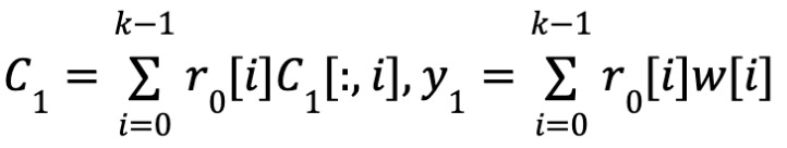
Consistency check: The processes of consistency check and proximity check are completely similar. The difference is that the random vector Y0 is not used but r0 is directly used to complete the linear combination part. Similarly, c1 is also a linear code for message y1, and has

ϕ(x)=. It is shown in [BCG 20 ] that, by consistency check, y=ϕ(x) holds with overwhelming probability if the committed matrix is ​​close to a codeword.

In pseudocode form, we give the flow of the Brakedown protocol:

Public input：The evaluation point X，parsed as a tensor product X=r0 ⊗r1 ;

Private input：The polynomial ϕ ，the coefficient of is denoted by w.

Let C be the [n, k, d]-limear code，EC：FkFn be the encoding function，N=k×k. If N is not a perfect square，we can pad it to the next perfect square. We use a python style notationmat[:, i] to select the i-th column of a matrix mat。

1. function PC. Commit(ϕ)：

2. Parse w as a k×k matrix. The prover locally computes the tensor code encoding C1 ，C2  ，C1 is a k×n matrix，C2 is a n×n matrix.

3. for i∈ [n] do

4. Compute the Merkle tree root Roott=Merkle.Commit(C2 [:, i])

5. Compute a Merkle tree root R=Merkle.Commit([Root0 ,......Rootn-1 ]), and output R as the commitment.

6. function PC. Prover(ϕ, X, R)

7. The prover receives a random vector Y0 ∈Fk from the verifier

8. Proximity 

   

9. Consistency  

   

10. Prover sends C1 , y1 , C0 , y0  to the verifier.

11. Verifier randomly samples t[n] as an array Î and send it to prover

12. for idx∈Î do

13. Prover sends C1  [:, idx] and the Merkle tree proof of Rootidx for C2  [:, idx] under R to verifier

14. function PC. VERIFY_EVAL(πX, X, y=ϕ(X), R)

15. Proximity: ∀idx∈Î, CY 0 [idx]==and EC(Yy 0 )==CY 0 

16. Consistency:∀idx∈Î, C1 [idx]==and EC(Y1 )==C1 

17. y==

18. ∀idx∈Î, EC(C1 [:, idx]) is consistent with ROOTidx, and ROOTidx’s Merkle tree proof is valid.

19. Output accept if all conditions above holds. Otherwise output reject.

references

references

1. [GLS+]:Alexander Golovnev, Jonathan Lee, Srinath Setty, Justin Thaler, and Riad S. Wahby. Brakedown: Linear-time and post-quantum snarks for r 1 cs. Cryptology ePrint Archive. https://ia.cr/2021/1043.

2. [XZS 22 ]:Xie T, Zhang Y, Song D. Orion: Zero knowledge proof with linear prover time[C]//Advances in Cryptology–CRYPTO 2022: 42 nd Annual International Cryptology Conference, CRYPTO 2022, Santa Barbara, CA, USA, August 15 – 18, 2022, Proceedings, Part IV. Cham: Springer Nature Switzerland, 2022: 299-328.https://eprint.iacr.org/2022/1010 

3. [BCG 20 ]:Bootle, Jonathan, Alessandro Chiesa, and Jens Groth. "Linear-time arguments with sublinear verification from tensor codes." Theory of Cryptography: 18 th International Conference, TCC 2020, Durham, NC, USA, November 16 – 19, 2020, Proceedings, Part II 18. Springer International Publishing, 2020.

4. Justin Thaler from A16z crypto, Measuring SNARK performance: Frontends, backends, and the future https://a16z crypto.com/measuring-snark-performance-frontends-backends-and-the-future/

5. Introduction to tensor product: https://blog.csdn.net/chenxy_bwave/article/details/127288938