Continuing from the previous chapter, we have published four articles in the series of articles on Building a Powerful Crypto-Asset Portfolio Using Multi-Factor Models:Theoretical Basics、Data Preprocessing、Factor Validity Test、Large Category Factor Analysis: Factor Synthesis。

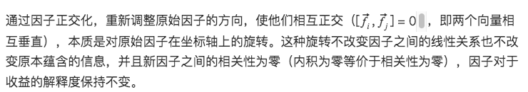
In the previous article, we explained in detail the problem of factor collinearity (high correlation between factors). Before synthesizing large categories of factors, factor orthogonalization needs to be performed to eliminate collinearity.

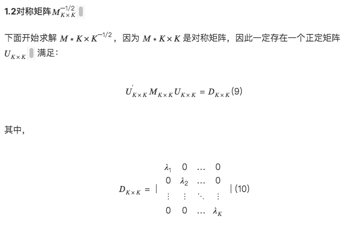
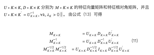
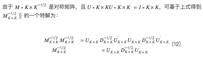
1. Mathematical derivation of factor orthogonalization

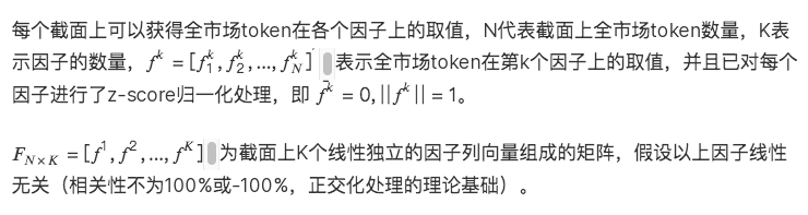
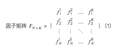
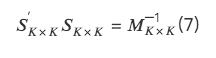
From the perspective of multi-factor cross-sectional regression, a factor orthogonal system is established.

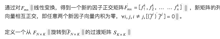
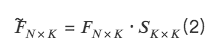
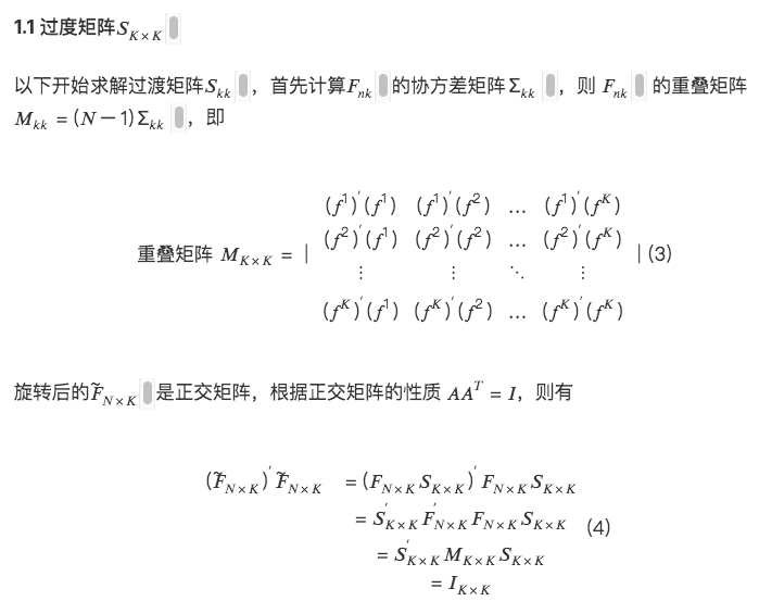
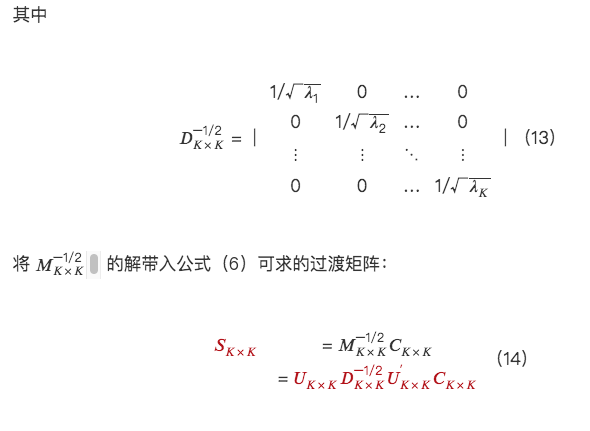
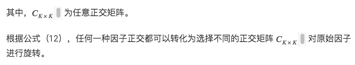
so,

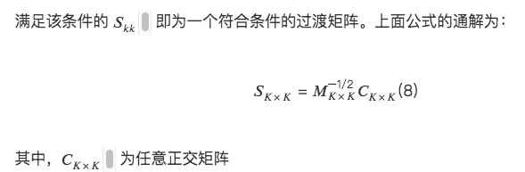
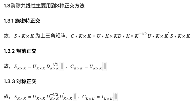
2. Specific implementation of three orthogonal methods

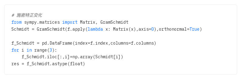
1.Schmitt orthogonality

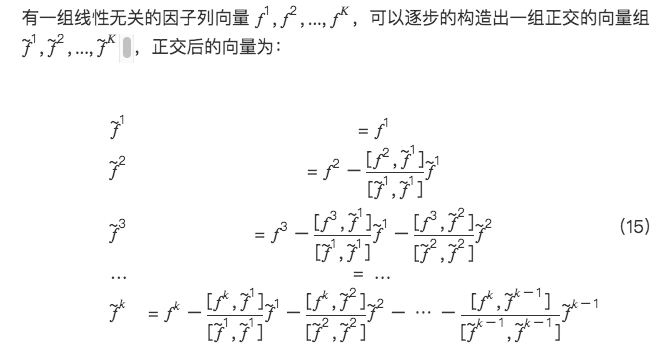
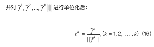
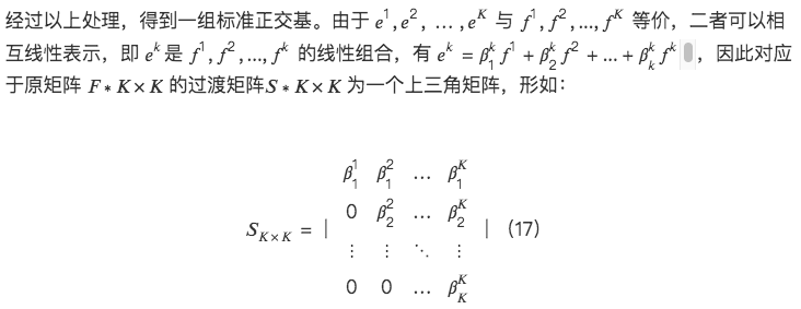
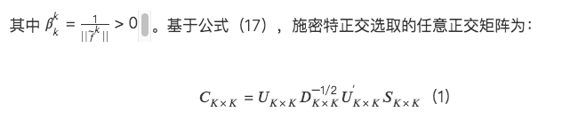
Schmidt orthogonal is a sequential orthogonal method, so it is necessary to determine the order of factor orthogonality. Common orthogonal orders include fixed order (the same orthogonal order is taken on different sections), and dynamic order (the same orthogonal order is taken on each section). The orthogonal order is determined according to certain rules). The advantage of the Schmidt orthogonal method is that there is an explicit correspondence between orthogonal factors in the same order. However, there is no unified selection standard for the orthogonal order. The performance after orthogonalization may be affected by the orthogonal order standard and window period parameters. .

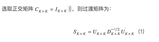
2.Normal orthogonality

# Canonical orthogonal def Canonical(self):
 overlapping_matrix = (time_tag_data.shape[ 1 ] - 1) * np.cov(time_tag_data.astype(float))
# Get eigenvalues ​​and eigenvectors
 eigenvalue, eigenvector = np.linalg.eig(overlapping_matrix)
# Convert to matrix in np
 eigenvector = np.mat(eigenvector)
 transition_matrix = np.dot(eigenvector, np.mat(np.diag(eigenvalue ** (-0.5))))
 orthogonalization = np.dot(time_tag_data.T.values, transition_matrix)
 orthogonalization_df = pd.DataFrame(orthogonalization.T, index = pd.MultiIndex.from_product([time_tag_data.index, [time_tag]]), columns=time_tag_data.columns)
 self.factor_orthogonalization_data = self.factor_orthogonalization_data.append(orthogonalization_df)

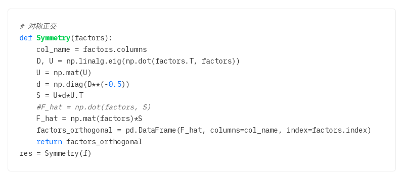
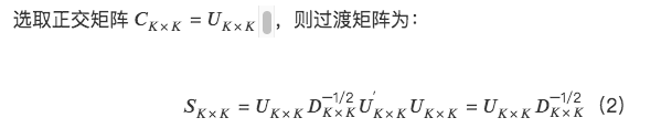
3. Symmetrical orthogonal

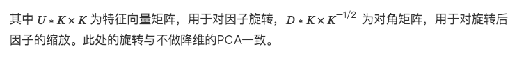
Since Schmidt orthogonal adopts the same orthogonal order of factors on several past sections, there is an explicit correspondence between the orthogonal factors and the original factors, while the canonical orthogonal selects the principal components on each section. The directions may be inconsistent, resulting in no stable correspondence between factors before and after orthogonality. It can be seen that the effect of the orthogonal combination depends largely on whether there is a stable correspondence between the factors before and after orthogonality.

Symmetric orthogonality reduces modifications to the original factor matrix as much as possible to obtain a set of orthogonal bases. This can maintain the similarity between the orthogonal factors and the causal factors to the greatest extent. And avoid favoring factors earlier in the orthogonal order like Schmidts orthogonal method.

Symmetric orthogonal properties:

1. Compared with Schmidt orthogonal, symmetric orthogonal does not need to provide an orthogonal order and treats each factor equally.

2. Among all orthogonal transition matrices, the similarity between the symmetric orthogonal matrix and the original matrix is ​​the greatest, that is, the distance between the before and after orthogonal matrices is the smallest.