Original author: Steven Wang

"What I cannot create, I do not understand."

-Richard Feynman

Introduction

You embrace Stable Diffusion and MidJourney to create magnificent images.

You skillfully use ChatGPT and LLaMa to compose eloquent texts.

You switch back and forth between MuseNet and MuseGAN to create beautiful music.

There's no doubt that the most unique ability of humans is to create, but in today's rapidly developing world of technology, we create through machines! Machines can generate original artwork in a given style (draw), write long coherent articles (write), compose pleasing music (compose), and even devise winning strategies for complex games (play). This technology is called Generative Artificial Intelligence (GenAI), and now is the best time to learn about GenAI.

1. Generative and Discriminative Models

GenAI is a buzzword that fundamentally refers to generative models, a branch of machine learning that aims to train models to generate new data similar to a given dataset.

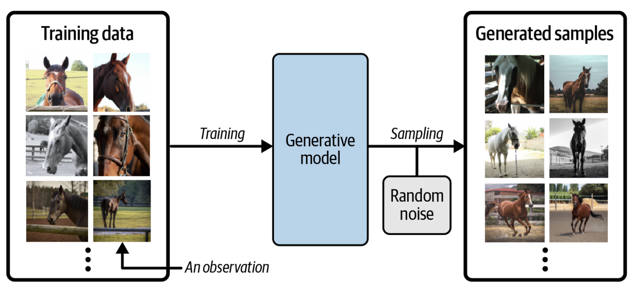
Let's say we have a dataset of horses. First, we can train a generative model on this dataset to capture the complex relationships between pixels in horse images. Then, we can sample from this model to create realistic horse images that don't exist in the original dataset, as shown in the following image:

In order to truly understand the objective and importance of generative models, it is necessary to compare them with discriminative models. In fact, most of the problems in machine learning are solved by discriminative models, as seen in the following example.

Let's say we have a dataset of paintings, some of which were painted by Van Gogh and others by other artists. With enough data, we can train a discriminative model to predict whether a given painting was created by Van Gogh. The process is illustrated in the following figure.

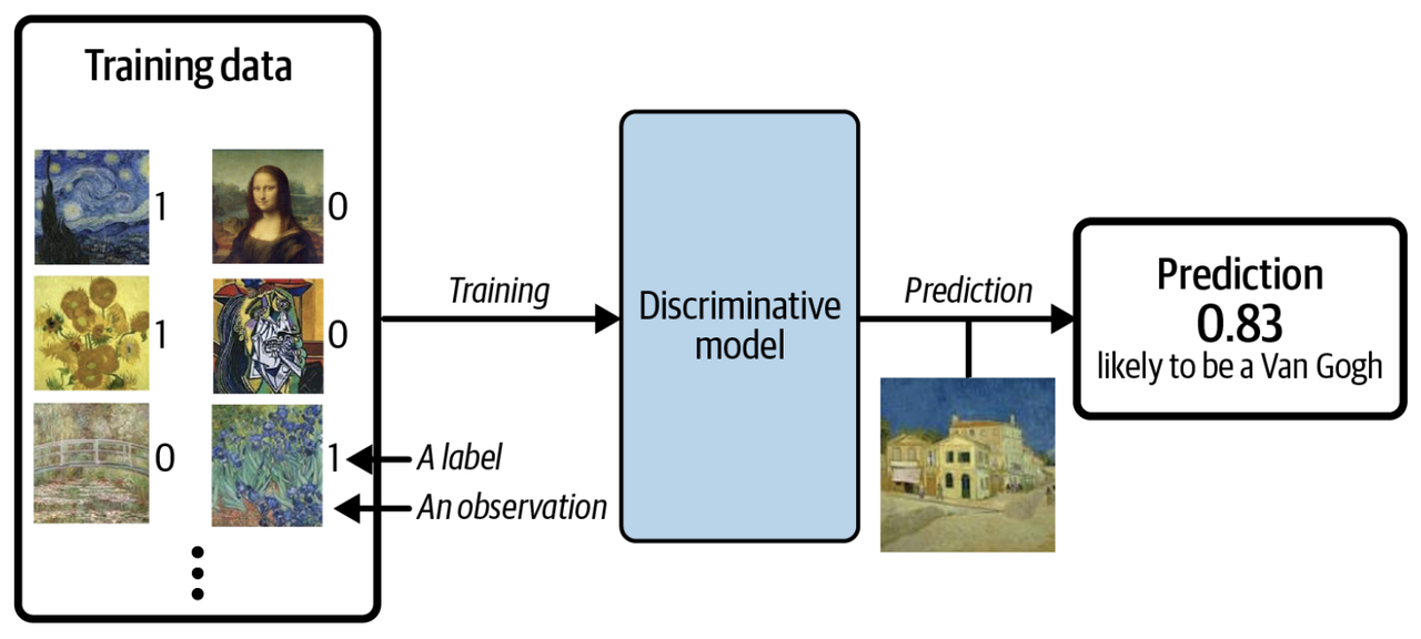
When using a discriminative model, each example in the training set has a label. For the binary classification problem described above, the label for Van Gogh's paintings is typically 1, and for non-Van Gogh paintings it is 0. In the image above, the model's final predicted probability is 0.83, suggesting a high likelihood that the painting was created by Van Gogh. Unlike discriminative models, generative models do not require labels in the examples because their goal is to generate new data, not predict labels for existing data.

Now that we've seen an example, let's use mathematical symbols to precisely define generative and discriminative models:

• A discriminative model models P(y|x), meaning it estimates the conditional probability of a label y given features x.

• A generative model models P(x), meaning it directly estimates the probability of features x and can sample new features from this probability distribution.

It is important to note that even if we were able to build a perfect discriminative model to identify Van Gogh's paintings, it still wouldn't know how to create a painting that looks like Van Gogh's. It can only output a probability, indicating the likelihood of the image being from the hand of Van Gogh. This illustrates that generative models are much more challenging than discriminative models.

2. Framework of Generative Models

Before understanding the framework of generative models, let's play a game. Assume the points in the figure below are generated according to a certain rule called Pdata. Now, your task is to generate a different x = (x 1, x 2) that makes this point appear to be generated by the same rule Pdata.

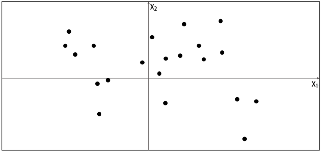
How do you generate this point? You may use the given points to create a model Pmodel in your mind, and this model represents the possible positions where the points can be generated. Therefore, the model Pmodel is an estimation of the model Pdata. The simplest model Pmodel is depicted as the orange box in the following diagram, where the points can only be generated inside the box and not outside the box.

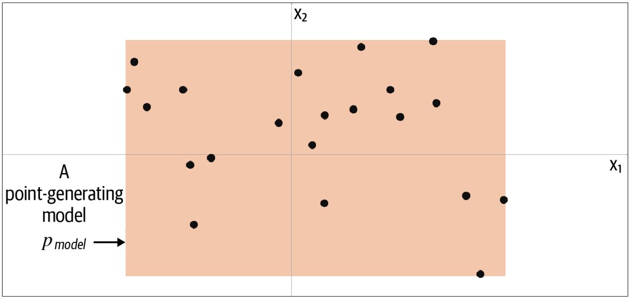
To generate new points, we can randomly select a point from inside the box or, more rigorously, sample from the distribution of the model Pmodel. This is a minimalistic generative model. You create a model (orange box) from the training data (black points), and then you can sample from the model, hoping that the generated points will resemble the points in the training set.

Now we can formally present the framework of generative learning.

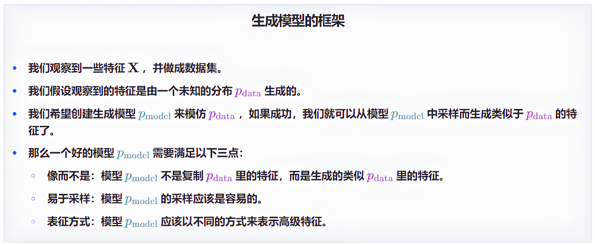
Now let's reveal the real data generating distribution Pdata and understand how to apply the above framework to this example. From the diagram below, we can see that the data generating rule Pdata is such that the points are uniformly distributed on land and not in the ocean.

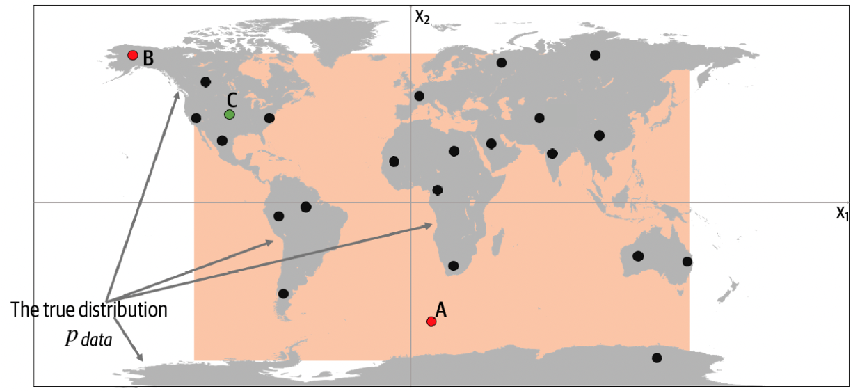
Obviously, our model Pmodel is a simplification of the rule Pdata. Examining points A, B, and C in the diagram can help us understand whether the model Pmodel successfully imitates the rule Pdata.

• Point A does not comply with the rule Pdata, as it appears in the sea, but it may be generated by the model Pmodel since it appears within the orange frame.

• Point B cannot be generated by the model Pmodel, as it appears outside the orange frame, but it complies with the rule Pdata, as it appears on land.

• Point C is generated by the model Pmodel and also complies with the rule Pdata.

This example demonstrates the basic concepts behind generative modeling. While generating models is much more complex in reality, the basic framework remains the same.

3. The First Generative Model

Suppose you are the Chief Fashion Officer (CFO) of a company, and your responsibility is to create new fashionable clothing. This year, you received 50 datasets on fashion combinations (as shown in the image below), and you need to create 10 new fashion combinations.

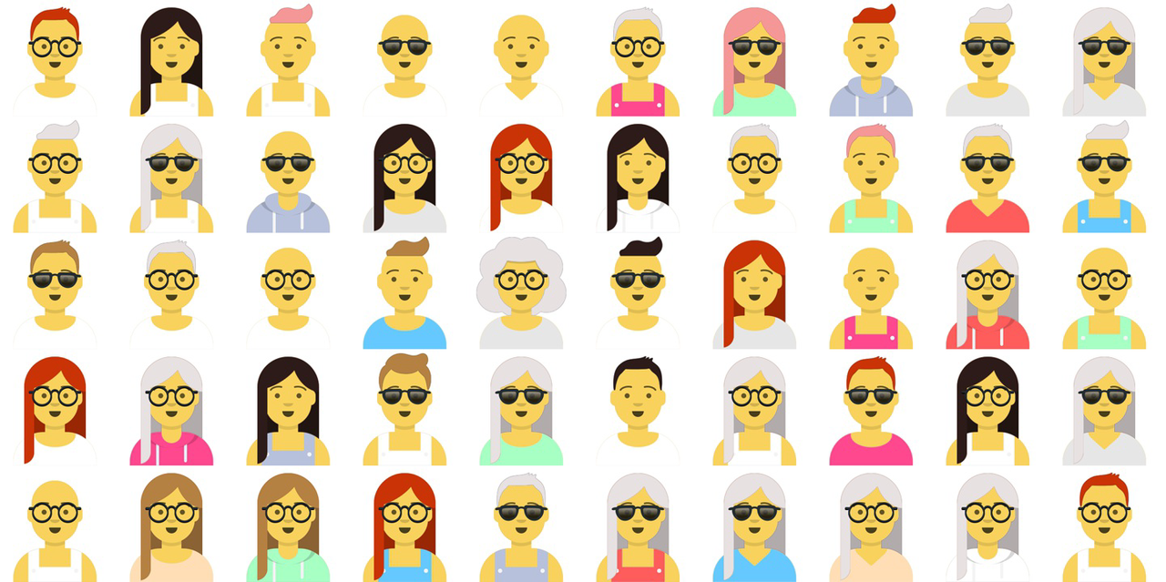
Although you are the Chief Fashion Officer, you are also a data scientist, so you decide to solve this problem using a generative model. After reviewing the 50 images above, you decide to describe fashion combinations using five features: accessories type, clothing color, clothing type, hair color, and hair type.

The first 10 image data features are as follows:

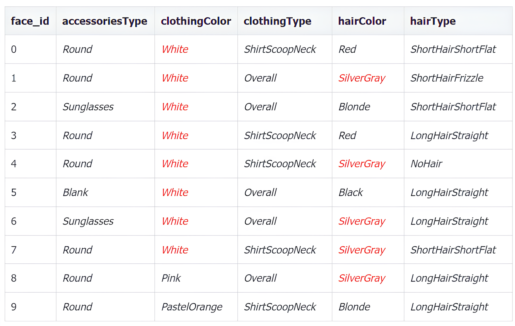
Each feature also has different values:

• 3 types of accessories type:

  Blank, Round, Sunglasses

• 8 types of clothing color:

  Black, Blue 01, Gray 01, PastelGreen, PastelOrange, Pink, Red, White

• 4 types of clothing type:

  Hoodie, Overall, ShirtScoopNeck, ShirtVNeck

• 6 types of hair color:

  Black, Blonde, Brown, PastelPink, Red, SilverGray

• 7 types of hair type:

  NoHair, LongHairBun, LongHairCurly, LongHairStraight, ShortHairShortWaved, ShortHairShortFlat, ShortHairFrizzle

There are 3 * 8 * 4 * 6 * 7 = 4032 possible feature combinations, so it can be considered that the sample space contains 4032 data points. From the given 50 data points, it can be observed that Pdata prefers certain feature values. From the table above, it can be seen that there are more white clothing colors and silver-gray hair colors in the images. Since we don't know the true Pdata, we can only build a Pmodel based on these 50 data points to make it similar to Pdata.

3.1 Simple Model

One simple method is to assign a probability parameter to each of the 4032 data points, which means the model will have 4031 parameters since the sum of all probability parameters equals 1. Now, let's check each of the 50 data points one by one and update the parameters of this model (θ 1 ，θ 2 ，…，θ 4031 ). The expression for each parameter is as follows:

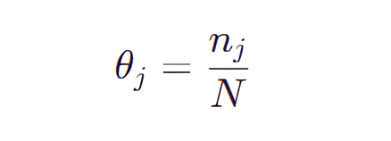
Where N is the number of observed data, which is 50, and nj is the number of occurrences of the j-th feature combination in the 50 data points.

For example, if the feature combination (LongHairStraight, Red, Round, ShirtScoopNeck, White) (referred to as combination 1) appears twice, then

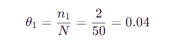
If the feature combination (LongHairStraight, Red, Round, ShirtScoopNeck, Blue 01) (referred to as combination 2) does not appear, then

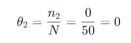
According to the above rule, we calculate a θ value for all 4031 combinations. It's not difficult to see that many θ values are 0. Even worse, it is impossible for us to generate new unseen images (θ = 0 means that no image with that combination of features has been observed). To solve this problem, we just need to add the total number of features (d) to the denominator and add 1 to the numerator. This technique is called Laplace smoothing.

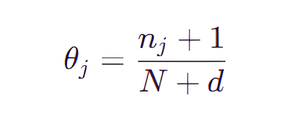
Now, each combination (including those not present in the original dataset) has a non-zero sampling probability. However, this is still not a satisfactory generative model because the probability of points not in the original dataset is a constant. If we try to use such a model to generate Van Gogh's paintings, it will operate with the same probability on the following two types of paintings:

1. Replicas of Van Gogh's original works (not in the original dataset)

2. Randomly assembled pixel art (not in the original dataset)

This is obviously not the generative model we want. We hope that it can learn some inherent structures from the data, so as to increase the probability weights of the regions in the sample space that it deems more likely, rather than placing all the probability weights on the points in the dataset.

3.2 Subtle Model

The Naive Bayes model can greatly reduce the frequencies of the above feature combinations, based on its model assumption that each feature is independent of each other. Going back to the data mentioned above, a person's hair color (feature xj) and their clothing color (feature xk) are not related, expressed mathematically as:

p(xj | xk) = p(xk)

With this assumption, we can calculate

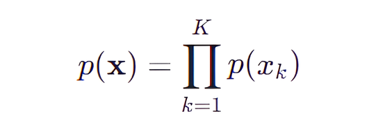
The Naive Bayes model simplifies the original problem of "estimating the probability for each feature combination" to "estimating the probability for each feature". Instead of needing 4031 (3 * 8 * 4 * 6 * 7) parameters, we only need 23 (3 + 8 + 4 + 6 + 7) parameters. The expression for each parameter is:

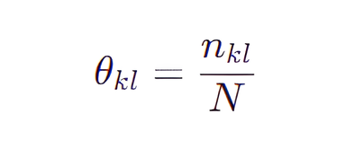
where N is the number of observed data, in this case, it is 50. nkl is the count of the lth feature value for the kth feature.

By analyzing the 50 data, the following table provides the parameter values for the Naive Bayes model.

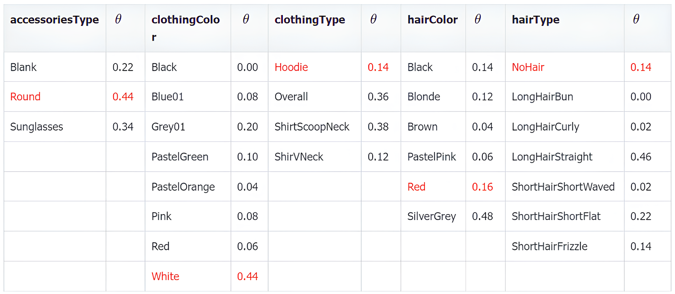
To calculate the probability of generating a certain data feature using the model, simply multiply the probabilities from the table, for example:

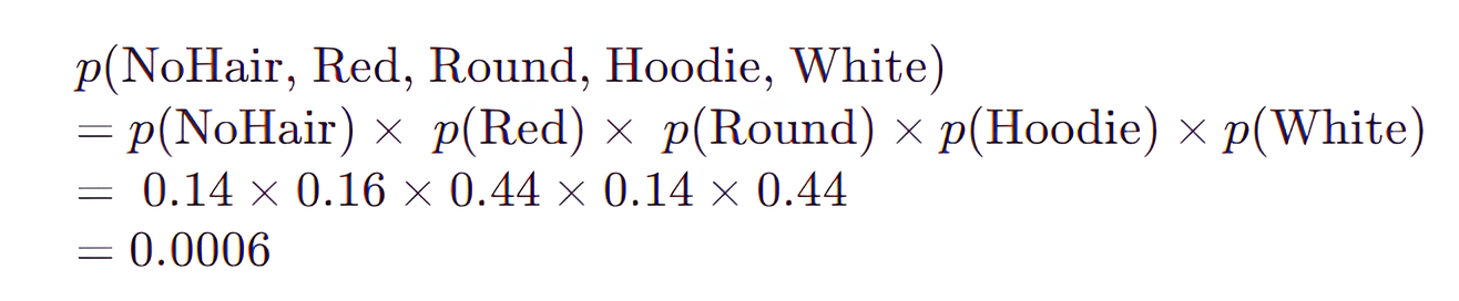
In this example, the combination does not appear in the original dataset, but the model still assigns a non-zero probability to it, allowing the model to generate it. Therefore, the Naive Bayes model can learn some structure from the data and use it to generate new examples that are not seen in the original dataset. The following image shows 10 new fashion pairing images generated by the model.

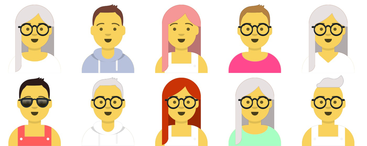
In this question, there are only 5 features belonging to low-dimensional data, and it is reasonable for the Naive Bayes model to assume that they are independent of each other. Therefore, the results generated by the model are good. Now let's take a look at an example of model collapse.

4. Challenges of Generative Models

4.1 High-Dimensional Data

As the Chief Fashion Officer, you have successfully generated 10 new fashion combinations using Naive Bayes. You were confident and thought your model was unbeatable, until you encountered the following dataset.

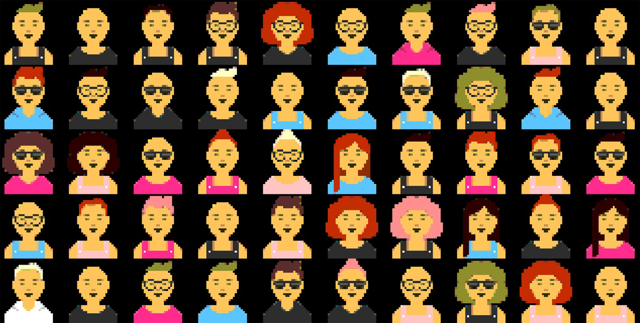
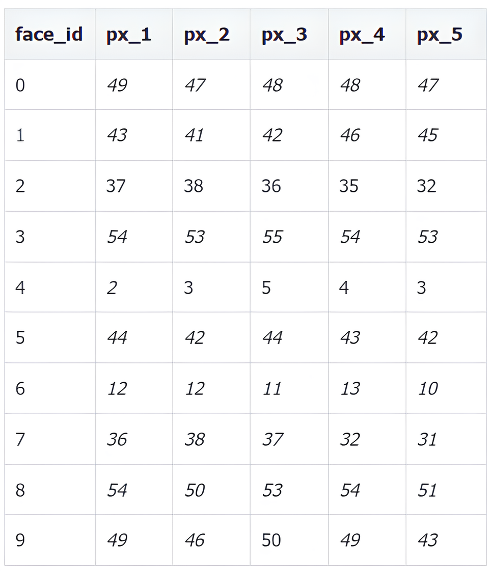
This dataset is no longer represented by five features, but by 32*32 = 1024 pixels. Each pixel value can be one of 0 to 255, where 0 represents white and 255 represents black. The table below shows the values of pixels 1 to 5 for the first 10 images.

Using the same model to generate 10 new fashion combinations, the following are the results of the model. Each image is equally ugly and it's impossible to distinguish different features. Why is this happening?

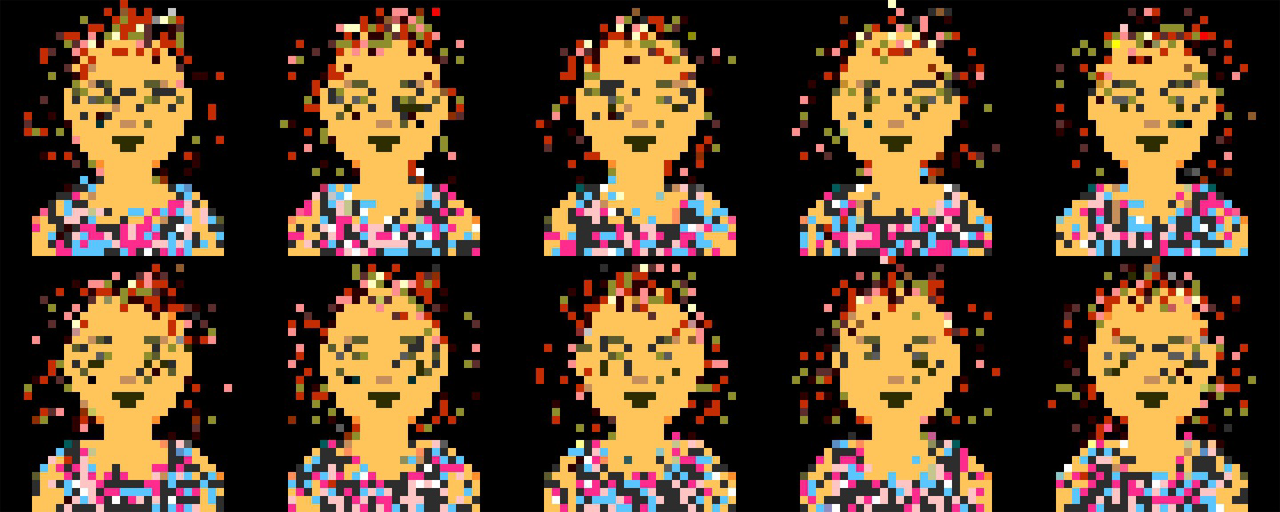
First of all, since the Naive Bayes model independently samples pixels, adjacent pixels are actually very similar. For clothing, the pixels should be roughly the same, but the model randomly samples, resulting in colorful clothes in the above image. Secondly, there are too many possibilities in the high-dimensional sample space, and only a small portion of them are recognizable. If the Naive Bayes model directly handles these highly correlated pixel values, the chances of finding satisfactory value combinations are very small.

In summary, for low-dimensional sample spaces with low correlated features, the Naive Bayes model works well with the effect generated by independent sampling. However, for high-dimensional sample spaces with highly correlated features, it is almost impossible to find effective face combinations through independent sampling of pixels.

This example emphasizes the two difficulties that a generative model must overcome to be successful:

1. How does the model handle conditional dependencies between high-dimensional features?

2. How does the model find the minimal proportion of observed results that satisfy the conditions from a high-dimensional sample space?

In order for a generative model to succeed in a high-dimensional and highly correlated feature sample space, it must utilize deep learning models. We need a model that can infer the relevant structures from the data, rather than being told to make certain assumptions in advance. Deep learning can form its own features in a low-dimensional space, which is a form of representation learning.

4.2 Representation Learning

Representation learning is about learning the meaning of high-dimensional data representations.

Suppose you meet an online friend you've never met before, and when you arrive at the agreed location, you can't find her because there are many people there. You call her and describe your appearance over the phone. I believe you wouldn't say the color of pixel 1 in the image is black, the color of pixel 2 is dark black, the color of pixel 3 is gray, and so on. Instead, you would assume that your online friend has a general understanding of what an ordinary person looks like, and then you would describe the features of the pixel group based on that understanding, such as having shiny black short hair, and wearing a pair of shiny glasses, etc. Usually, with no more than 10 such descriptions, your online friend can generate an image of you in her mind. The image may be rough, but it doesn't prevent her from finding you among hundreds of people, even though she has never seen you before.

This is the core idea behind representation learning: instead of trying to directly model the high-dimensional sample space, use a low-dimensional latent space to describe each observation in the training set. Then learn a mapping function that can take a point from the latent space and map it to the original sample space. In other words, each point in the latent space represents the features of high-dimensional data.

If the above explanation is not easy to understand, please refer to the following figure, which shows a training set consisting of grayscale jar images:

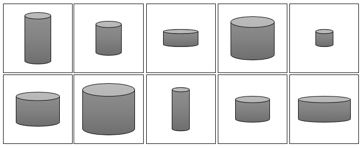
It is not difficult to see that these jars can be described by only two features: height and width. Therefore, we can convert the high-dimensional pixel space of the image into a two-dimensional latent space, as shown in the following figure. In this way, we can sample from the latent space (blue dots) and then convert them into images through a mapping function f.

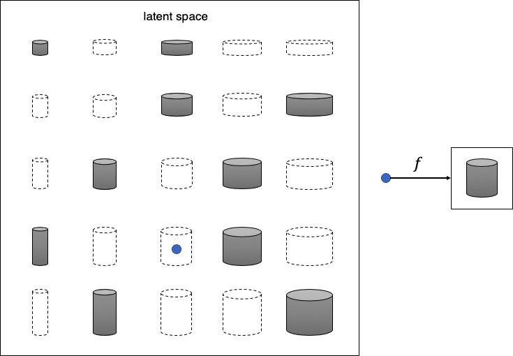
It is not easy for a machine to realize that the original dataset can be represented by a simpler latent space. First, the machine needs to determine that height and width are the two latent space dimensions that best describe this dataset. Then, it learns the mapping function f  that can take a point in this space and map it to a grayscale jar image. Deep learning allows us to train machines to find these complex relationships without human guidance.

5. Classification of Generative Models

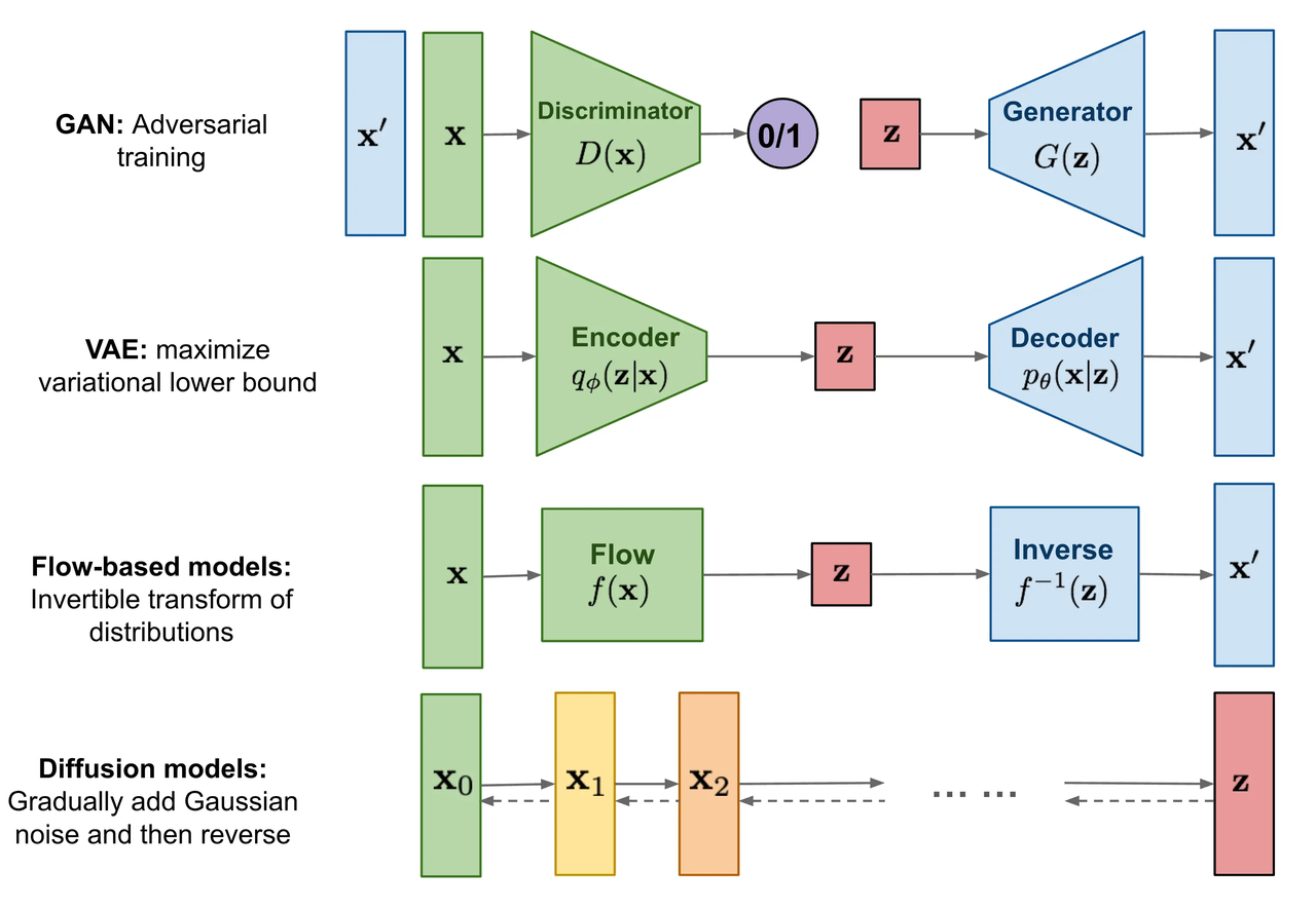
All types of generative models aim to solve the same task, but they have slightly different approaches to modeling the density function. Generally, there are two categories:

• Explicit modeling of the density function,

  but with some constraints to compute the density function, such as normalizing FLOW model.

  Approximating the density function, such as variational autoencoder (VAE) and diffusion model.

• Implicit modeling of the density function by directly generating the data through a random process, such as generative adversarial network (GAN).

Summary

Generative Artificial Intelligence (GenAI) is an artificial intelligence that can be used to create new content and ideas (including text, images, videos, and music). Like all artificial intelligence, GenAI is a large-scale model that is pre-trained by deep learning models based on a large amount of data, often referred to as the foundation model (FM). With GenAI, we can create more stunning images, write more beautiful texts, and compose more moving music, but the first step is to understand how GenAI creates new things, as Richard Feynman said, "I can't understand something I can't create."