






SignalPlus: A Discussion on Deep Neural Networks


Author: Steven Wang
Deep neural networks are completely flexible by design, and there really are no fixed rules when it comes to model architecture.
-- David Foster

Introduction
Neural network is inspired by the human brain and can simulate the signaling between biological neurons. A neural network is a system composed of neurons. As shown in the diagram below, a neuron has many dendrites for input and one axon for output. It has two main characteristics: excitability and conductivity:
Excitability refers to the fact that when the stimulus intensity does not reach a certain threshold, the neural impulse does not occur; but when the stimulus intensity reaches that value, the neural impulse occurs and can reach maximum intensity instantaneously.
Conductivity refers to the fact that adjacent neurons transmit through a small gap between them. This small gap, called a synapse, functions to transmit neural impulses between different neurons. The synapse in the diagram below connects neuron A and B.
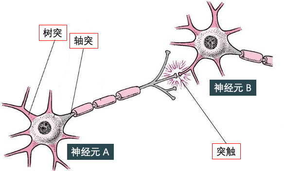
Imagine many synapses connecting many neurons, doesn't it form a neural network? That's right, in analogy to artificial neural network (ANN), it is also composed of countless artificial neurons, such as the shallow neural network and the deep neural network shown in the figures on the left and right below.
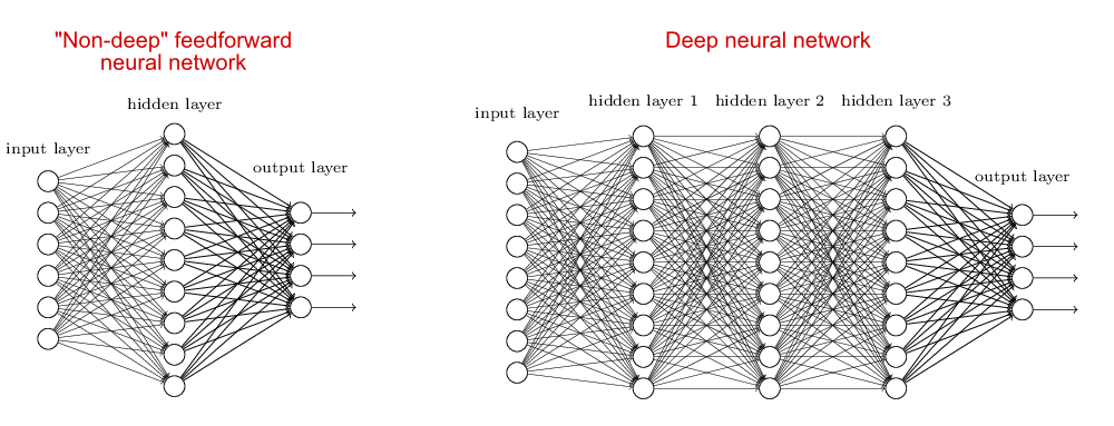
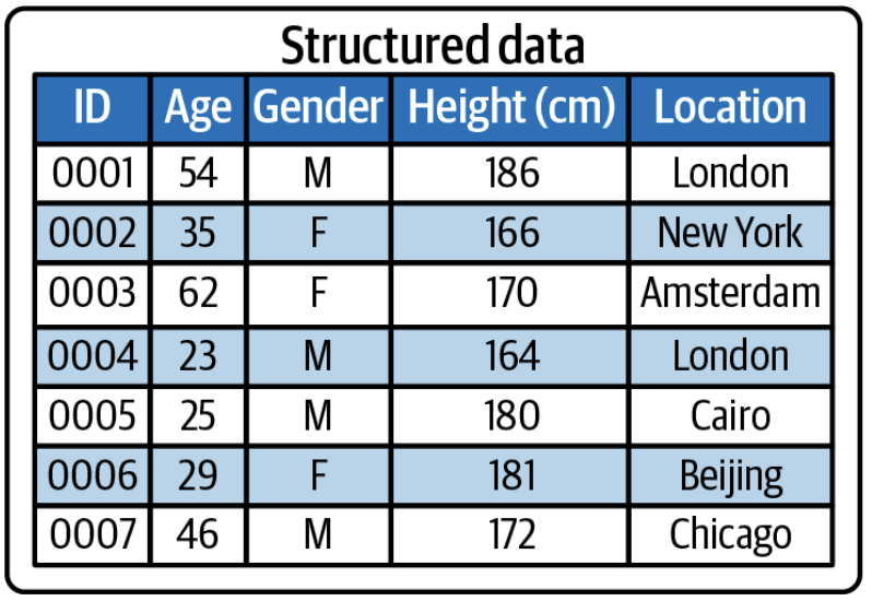
Shallow neural networks are suitable for structured data, such as two-dimensional data stored in Excel as shown in the picture below.
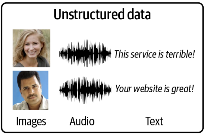
 Deep neural networks are suitable for unstructured data, such as images, texts, and speech data shown in the picture below.
Generative AI models mainly generate unstructured data, so understanding deep neural networks is necessary. Starting from this article, we will have both models and code flying together, because
Talk is cheap. Show me the code.
-- Linus Torvalds
We will implement the code using TensorFlow and Keras.

1. Artificial Neural Networks
1.1 Introduction to Neural Networks
Assuming the neural network below has been trained, it is then used to predict whether there is a smiling face in the picture.
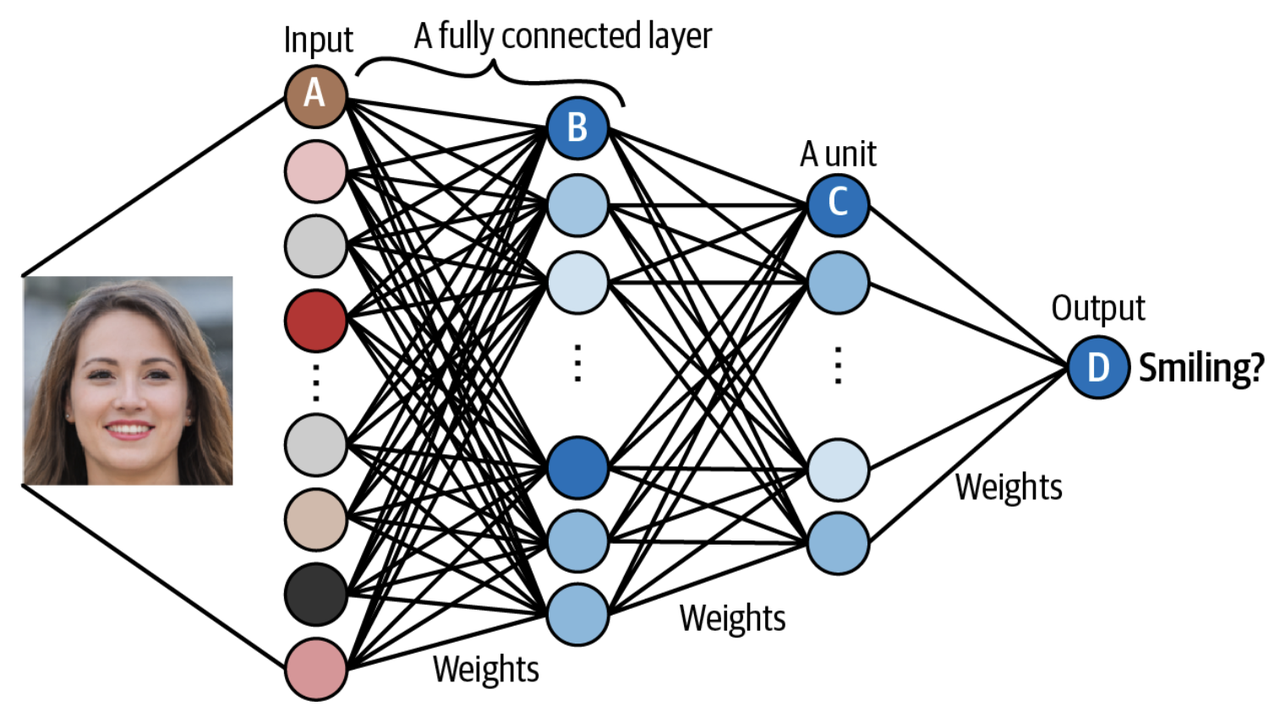
Unit A receives pixel information in the image.
Unit B combines input pixels and emits the strongest signal when there are low-level features such as edges in the original image.
Unit C combines low-level features and emits the strongest signal when there are high-level features such as teeth in the original image.
Unit D combines high-level features and emits the strongest signal when a person in the original image is smiling.
When this neural network is "fed" with enough data, namely images, it will "find" a set of weights that make the final predictions as accurate as possible. This process of finding weights is actually training the neural network.
After having a preliminary understanding of the neural network, the next task is to implement it using Keras.
1.2 Keras Training Process
In Keras, implementing a neural network involves understanding three key points:
Models
Layers, Inputs, and Outputs
Optimizer and Loss Function
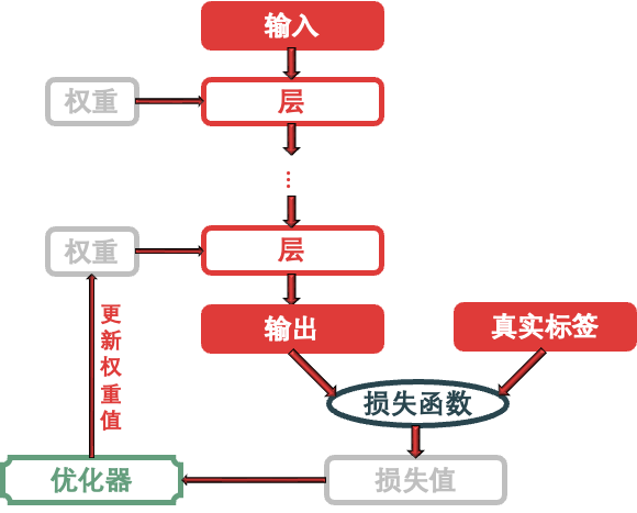
Summarizing the process of training a neural network in Keras with the above keywords: linking multiple layers together to form a model, mapping input data to predicted values. Then, the loss function outputs these predicted values and compares them with the target to obtain a loss value (which measures the degree of match between the network's predicted values and expected results), and the optimizer uses this loss value to update the network's weights.
Finally, I can show you some code here, even if it includes importing libraries. First, we use the module from the tensorflow.keras library to build a neural network.
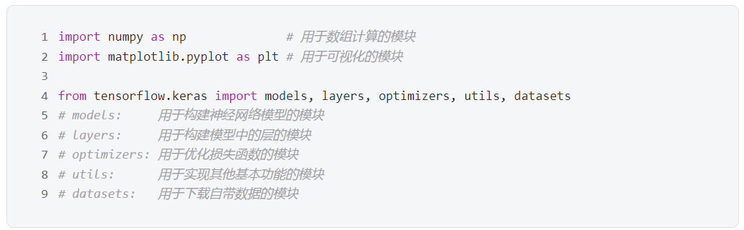
The whole neural network is a model, and the code for the main framework comes from the models module. The model is composed of multiple layers, and the code for different layers comes from the layers module. The first layer of the model is the input layer, which is responsible for receiving inputs. The last layer of the model is the output layer, which is responsible for providing outputs. Both the input and output layers are in the models module. Once the model structure is set, we need the optimizers module to train it.
1.3 Simple Neural Network
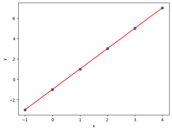
Students who have learned machine learning must have encountered their first model, which is linear regression, and to be more specific, uni-variate linear regression. Given a set of data of x and y:
x = [-1, 0, 1, 2, 3, 4]
y = [-3, -1, 1, 3, 5, 7]
We need to find the relationship between x and y. Given xnew = 10, what is ynew?
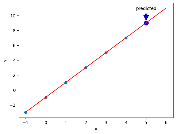
As shown in the graph below, we can plot the points of x and y, and it's not hard to find that the red line in the graph represents the relationship between x and y. Now, we want to use Keras, a powerful tool, to build a neural network to find this red line.
1.3.1 Creating the Model
We only need a neural network with one layer and one neuron. The code is as follows:

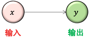
First, use models.Sequential () to create an empty neural network, and then continuously add layers. Here we add layers.Dense (), called a dense layer. The parameter input_shape=[ 1 ] in the function indicates that the dimension of the input data is 1, and units= 1 indicates that there is only 1 neuron in the output. The visualization is as follows:
1.3.2 Check the Model
Check the model information, strangely, the number of parameters (Param #) is 2 instead of 1. Because from the figure above, y = wx, there should only be one parameter, w.

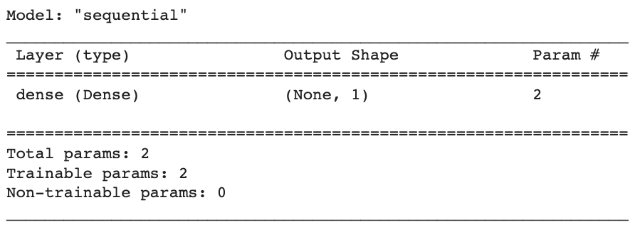
The reason is that when calculating the number of parameters for each layer, each neuron is connected to a bias unit with a value of 1 by default. Therefore, the more accurate representation of the figure above is as follows:
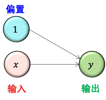
This is correct. At this time, y = wx+b, there are w and b two parameters.
Strictly speaking, there is actually a parameter called activation in the Dense() function, which literally means activation function, and essentially converts wx + b into y in a non-linear mode. If the activation function is defined as g, then y = g(wx + b). In Keras, if no value is specified for activation, no non-linear conversion is needed. With the concept of activation function, we provide a complete graph:
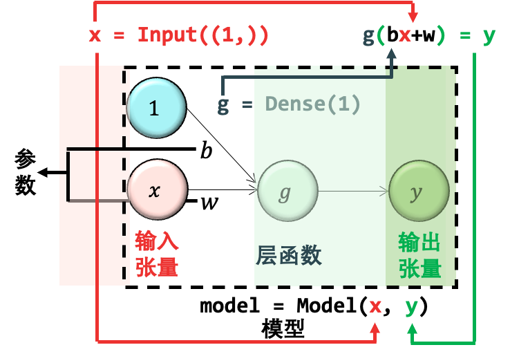
Our goal is to find the parameters in the graph, the weight w and the bias b.
1.3.3 Compile Model
After the model framework is built, the next step is to optimize the problem. In the following compile() function, the parameters optimizer="sgd" are set, which specifies the optimization method as stochastic gradient descent, and the parameter loss="mean_squared_error" specifies the loss function as mean squared error.

1.3.4 Train Model
The fit() function is used to train the model by passing in the data x and y. It is worth noting that the parameter epochs=500. In Chinese, epoch means the number of times the entire training set is traversed by the algorithm, and here it means the model training is performed for 500 epochs.

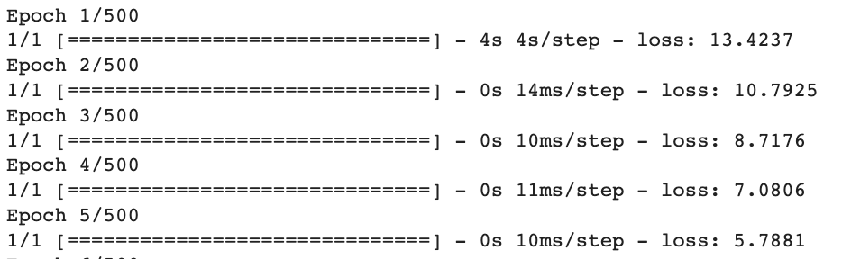
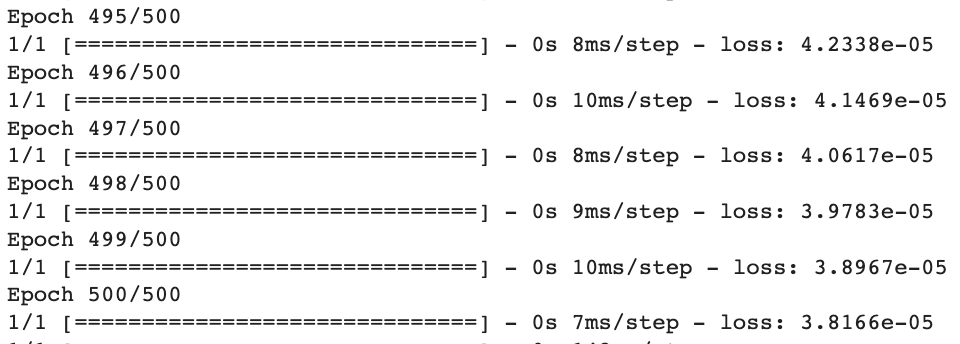
Printing out the information of the first and last 5 periods, it is not difficult to find that the initial loss is very high, 13.4237, and the final loss is very small, only 3.8166e-05, indicating that the predicted values and the true values in the training set are almost identical.
After model training, you can use the get_weights() function to check the parameters.
 The first result returned is the weight w, and the second is the bias b. Therefore, the neural network model is y = 1.9973876 x - 0.99190086 ≈ 2 x - 1.
1.3.5 Evaluate the Model
To evaluate the model, use the predict() function by passing in the new data x_new and obtaining the result 8.995028, which is very close to 2*x_new - 1 = 9.

From the graph below, it can be seen that the neural network has "learned" the model (red line) from 6 data points (deep cyan dots), and this model can be applied to new data (blue dots).
Summarize the whole process of neural networks:
Create model: Use Sequential(), of course there are other better methods, which will be discussed in the next section.
Check model: Use summary()
Compile model: Use compile()
Train model: Use fit()
Evaluate model: Use predict()
Although this example builds a minimalist neural network, it still consists of all five steps. Building a complex neural network also requires these five steps. The difference is that in step 1, when creating the model, many layers need to be concatenated, and in step 5, a more advanced optimizer needs to be selected. But the essence remains unchanged. In the next two sections, we will take a look at two slightly more complex neural networks, namely feedforward neural network (FNN) and convolutional neural network (CNN).
2. Feedforward Neural Network (FNN)
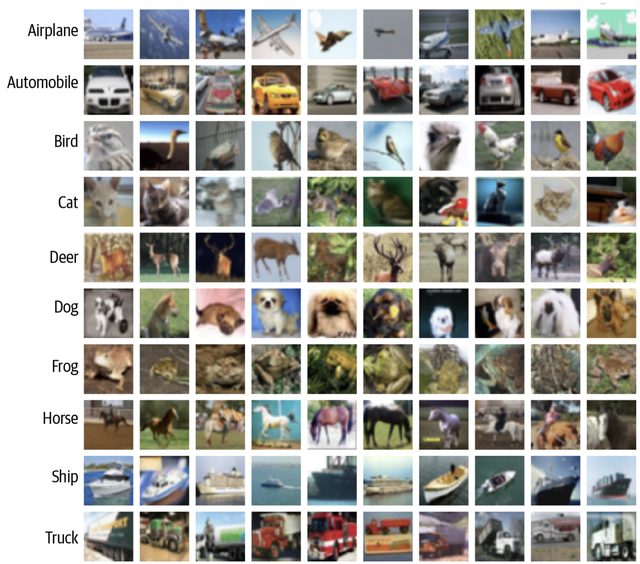
The minimalist neural network in the previous section was too boring, but its primary purpose is to clarify the concept of neural networks in Keras. Now, let's see what interesting things neural networks can do, like predicting image categories. First, let's take a look at the dataset used, CIFAR-10 (https://www.cs.toronto.edu/~kriz/cifar.html).
This dataset consists of 60,000 color images, each image is 32*32 pixels, divided into 10 categories with 6000 images per category. Among them, 50,000 images are used for training, and the other 10,000 are used for testing. The following image shows 10 randomly selected images from each category:
Use the load_data() function in the datasets module to download the data and normalize the pixel values of the images. The original pixel values range from 0 to 255, and now they are normalized to range from 0 to 1.

For the categories, use the to_categorical() function in the utils module to perform one-hot encoding. The idea is to represent the integers with a vector that contains only one 1. For example, after one-hot encoding, category 5 becomes [0, 0, 0, 0, 1, 0, 0, 0, 0, 0]. The vector has 10 elements, which is the same as the number of categories. Only the 5th element of the vector is 1 (hot), while the others are 0 (cold).

The first ten images of the training set are shown below:

2.1 Model Creation
2.1.1 Sequential
We have already seen how to build a sequential model in the previous section. First, create an empty neural network using models.Sequential(), and then add layers continuously. In this example, there is a flatten layer layers.Flatten() and three dense layers layers.Dense().
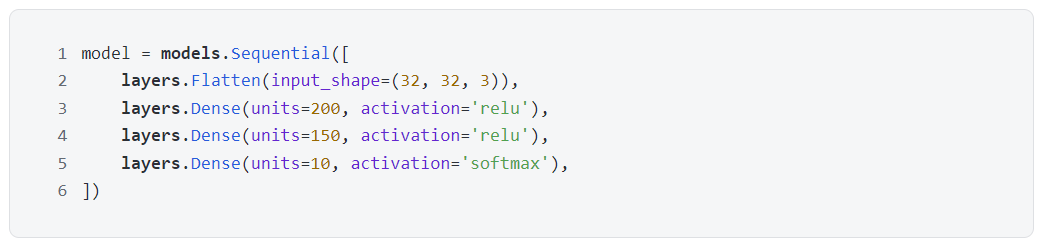
The above code gives the model shown in the figure below:
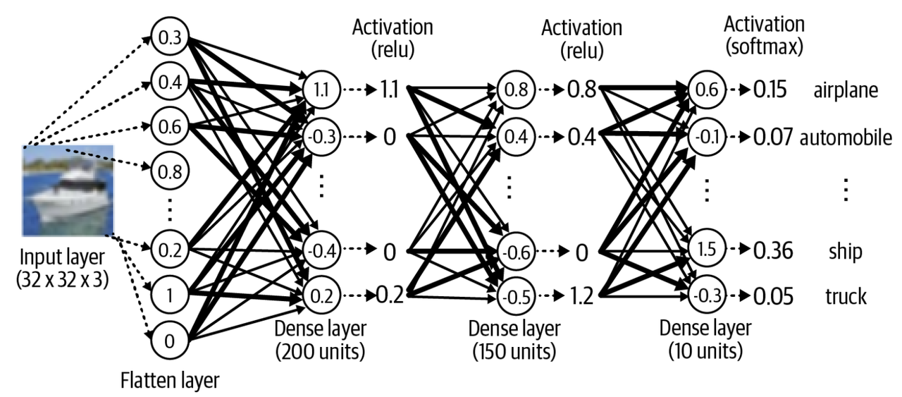
With the understanding of the percept, let's study the code again. Why do we need to flatten the layer? Because the image has three dimensions: width, height, and color channels, and the process of flattening to one dimension is shown in the figure below.
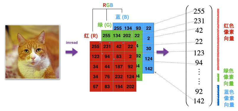
The original image ( 32, 32, 3) is flattened to a 32 * 32 * 3 = 3072 vector by the input flatten layer (the dimension of the image is specified in the parameter input_shape), which can be understood as having 3072 neurons as input. Then the three dense layers:
-
The number of neurons (parameter units) is 200, 150, and 10, respectively. The first two, 200 and 150, are given randomly or tuned as hyperparameters, but the last one, 10, is consistent with the number of classes.
-
The activation functions used (parameter activation) are relu, relu, and softmax, respectively. The first two relu's are almost standard, but the last softmax is task-specific. If it is a multi-classification problem, softmax is used.
The commonly used activation functions are shown in the figure below:
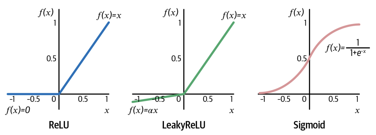
ReLU converts negative inputs (x < 0) to 0 and keeps positive inputs (x > 0) unchanged. LeakyReLU is very similar to ReLU, the only difference is that for negative inputs (x < 0), the converted result is also a negative number related to the input (ax).
Sigmoid converts real numbers into numbers between 0-1, which can be treated as probabilities. Therefore, the Sigmoid function is used for binary classification problems. Its extended version, Softmax, is used for multi-class classification problems.
2.1.2 Functional Approach
In practice, we are more accustomed to functional modeling. Models built using sequential approach can also be accomplished using functional approach, but not vice versa. If you have to choose between the two, it is recommended to only use functional approach to build models. The code is as follows:
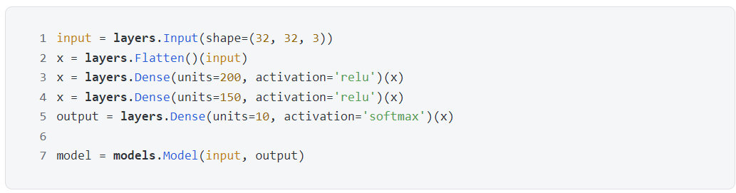
Remember this sentence when using functional approach for modeling: Treat layers as functions. With this sentence in mind, the code becomes easy to understand.
In line 1, use Input() to receive image data.
In line 2, treat Flatten() as function f, simplifying it to x = f(input)
In line 3, treat Dense(units=200, activation='relu') as function g, simplifying it to x = g(x)
In line 4, treat Dense(units=150, activation='relu') as function h, simplifying it to x = h(x)
The line 5, treating Dense(units= 10, activation='softmax') as function q, isn't simplifying it to output = q(x)
By passing input through layers of functions, the output is equal to q(h(g(f(input)))), and finally establishes the relationship using models.Model.
2.2 Model Check
After creating and before using the model, it is best to check the data shape of each layer in the neural network. This can be done using the summary() function, which will print out such information.

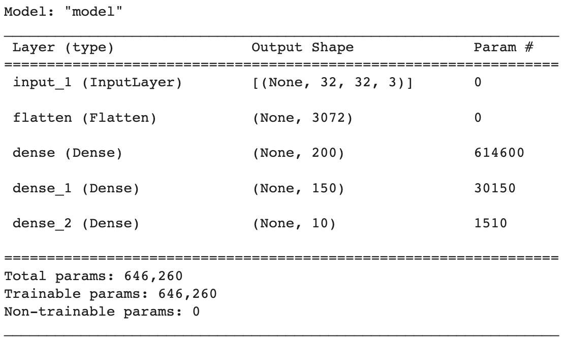
The model is automatically named "model", followed by a table describing the name type (layer (type)), output shape (Output Shape), and number of parameters (Param #) of each layer. Let's go through them layer by layer:
The InputLayer is named input_ 1 , with output shape [None, 32, 32, 3 ]. The last three elements correspond to the image width, height, and color channels. The first "None" actually represents the number of samples in a batch. To keep the code concise, this number of samples is usually not explicitly written when building the model.
The Flatten layer is named flatten, with 3072 being the number of elements after flattening 32x32x3. The number of parameters is 0 because flattening reshapes the array without requiring any parameters.
The first Dense layer is named dense, with an output shape of 200, and 614,600 parameters = (3072 + 1) * 200, don't forget about the bias units.
The second Dense layer is named dense_1, with an output shape of 150, and 30,150 parameters = (200 + 1) * 150, also considering the bias units.
The third Dense layer is named dense_2, with an output shape of 10, and 1,510 parameters = (150 + 1) * 10, also considering the bias units.
At the bottom, the total number of parameters (Total params) is 646,260, the number of trainable parameters (Trainable params) is 646,260, and the number of non-trainable parameters (Non-trainable params) is 0. Why are there parameters that don't need training? Well, think about transfer learning, where you lock the first n layers of a borrowed network and only train the last 1-2 layers. The parameters of the preceding n layers don't participate in training, do they?
2.3 Model Compilation
Once the model is built, we need to compile it by setting three things:
Select the loss function based on the task to be solved
Select the ideal optimizer
Select the metrics to be monitored
We use the complie() function to compile the model, as shown in the code below:
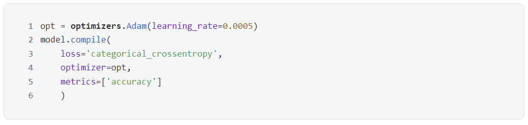
In the complie() function:
For the parameter loss, in this example is a ten-classification problem, so the loss function used is categorical_crossentropy. In addition:
For binary classification problems, the loss function is binary_crossentropy.
For regression problems, the loss function is mean_squared_error.
For the parameter optimizer, in most cases, using adam and rmsprop optimizers with their default learning rates is reliable. When setting this parameter, it can also be called by name or instantiated as an object.
Name: 'sgd'
Object: optimizers.Adam(learning_rate=0.0005)
For the parameter metrics, it can also be called by name or instantiated as an object. In this example, the metric is accuracy, so it can be written as
Name: ['accuracy']
Object: [metrics.categorical_accuracy]
Note that metrics do not affect the training process of the model, they only allow us to monitor the performance of the model during training. Only the loss function affects the training process of the model.
2.4 Train the model
Training the model is not done by throwing all the data together, but in batches. Before introducing training the model, a few concepts need to be clarified:
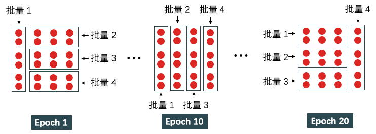
Batch size refers to the number of samples in a batch. In the example below, there are a total of 24 data points. If each batch contains 6 data points, then the total can be divided into 4 batches.
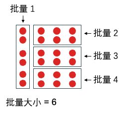
Epoch refers to one complete pass through the entire training dataset by the algorithm. When set to 20 epochs, the training dataset is traversed in different ways for 20 times. One epoch requires 4 iterations to traverse the entire dataset, which is equal to the total number of samples / batch size = 24 / 6 iterations. The process of running 20 epochs is shown in the figure below.
The fit() function is used to train the model, as shown in the code below:
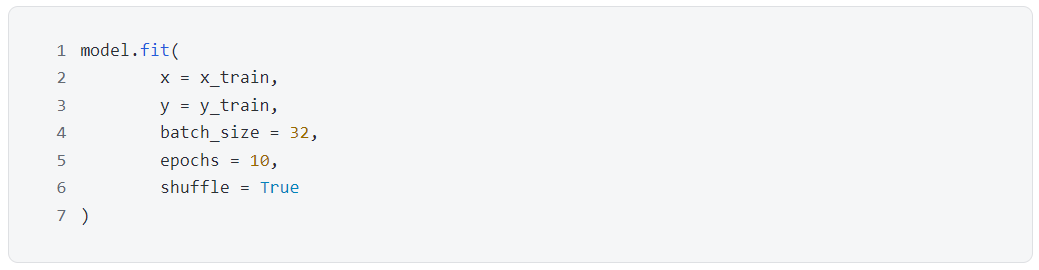
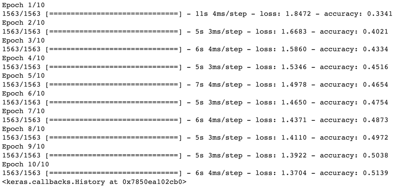
The training steps are shown in the figure above, and it is not difficult to see that the training set is divided into 1563 batches, with each batch containing 32 images (batch size). After 10 epochs, the loss function (categorical cross-entropy) decreased from 1.8472 to 1.3696, while the accuracy increased from 33.41% to 51.39%. The model can achieve an accuracy of 51.39% on the training set, but how will it perform on unseen data?
2.5 Evaluate the Model
Use the evaluate() function to directly view the accuracy.


The accuracy of the model on the test set is 49.52%, which is 10% higher than random guessing (due to the ten classes). Considering that we used a very simple feed-forward neural network to predict image categories, an accuracy of 49.52% is already considered a good result.
Use the predict() function to compare the predicted and true classes.
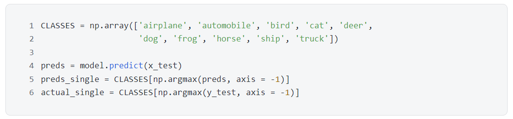
In the test set, there are 10,000 images and 10 classes, so the preds is an array of size [ 10000, 10 ], where each row represents the probabilities of the model's predictions for the 10 classes of the corresponding image. Of course, the sum of all probabilities is equal to 1. Let's take a look at the prediction results for the first image in the test set:


y_test is also a [10,000, 10] array, and each row represents the true class of the corresponding image, so there are 9 zeros and 1 one among the 10 elements. Let's see the true class of the first image in the test set:


It is not difficult to see that the probability of class four is the highest in the prediction results preds[0,:] with a value of 0.38579068, and the true class test[0,:] is indeed class four (with the fourth element being one). We will use np.argmax to find the indices of the maximum values in both the prediction results preds[0,:] and the true class test[0,:], and then map them to class descriptions using CLASSES.

The first image in the test set is a cat, and the model correctly predicts it to be a cat!
Now let's try the fourth image.

The fourth image in the test set is a ship, but the model predicts it to be an airplane, which is incorrect!
Visualization: The above method of comparison is too complicated. We can randomly select 10 images from the test set, print each image, and also display the predicted class and the true class below the image.
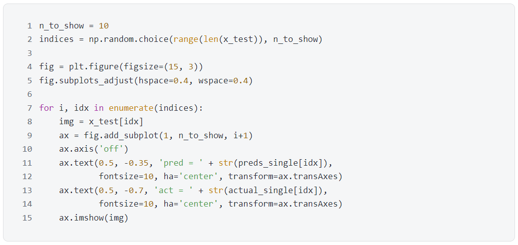

From the 10 small pictures above, it can be seen that the model correctly predicts 5 of them, with an accuracy rate of 50%, which is consistent with the previously calculated 49.52%. Although this is only a discriminative model used for prediction, the content discussed in this section (such as layers, activation functions, and optimizers) still apply when we create generative models.
Next, let's see how to improve the model using Convolutional Neural Networks (CNN).
3. Convolutional Neural Networks (CNN)
The fundamental reason why Feedforward Neural Networks (FNN) perform poorly on image classification problems is that they do not consider the spatial structure of images. For example, neighboring pixels in an image are very close to each other, but FNN initially flattens the pixels, destroying the unique spatial structure of images. We need a neural network that is more suitable for images, such as Convolutional Neural Networks (CNN).
3.1 Basic Concepts
Imagine that you are in the dark and a large picture appears in front of you. You cannot see that it's a car in the dark, so you have to use a flashlight to scan it bit by bit, projecting what you see each time onto the next layer, and so on. For example, in the first layer, you see some horizontal, vertical, and diagonal lines, in the second layer, they combine to form circles and squares, in the third layer, they combine to form wheels, doors, and the body of the car, and in the fourth layer, they combine to form a car. In this way, you can use a flashlight in the dark to identify if there's a car in the photo.
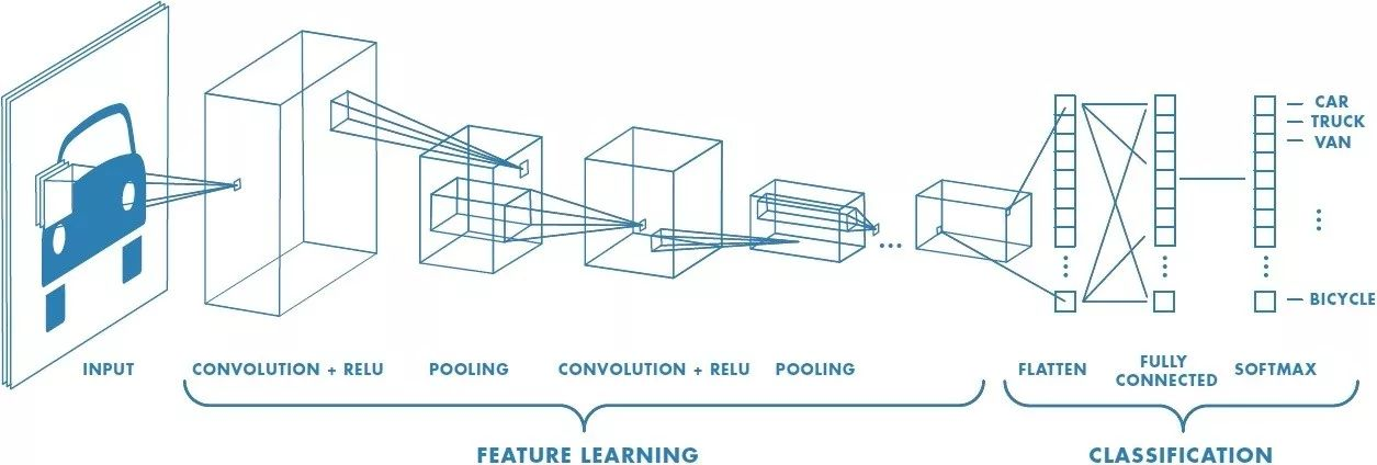
The above example is actually the process of a Convolutional Neural Network recognizing images. First, let's clarify a few definitions:
Filter: slides on the width and height of the input data, performs convolution with the input data, just like the flashlight in the example above.
Convolution: The definition here is to multiply all "filter pixels" by "pixels as the filter sweeps through the image" and then sum them up.
Stride: The stride of the filter when traversing the image. The default value is 1, which means the filter moves one pixel at a time.
Padding: Sometimes the input data is padded with zeros at the edges to control the size of the output data (commonly used to keep the size of the output data consistent with the input data).
Convolution
The most important feature of convolutional neural networks is the convolution operation. Recalling the above definition, we multiply the "filter pixels" by the "pixels as the filter sweeps through the image" and then sum them up. Take a look at the two examples below, assuming the filter size is 3x3.
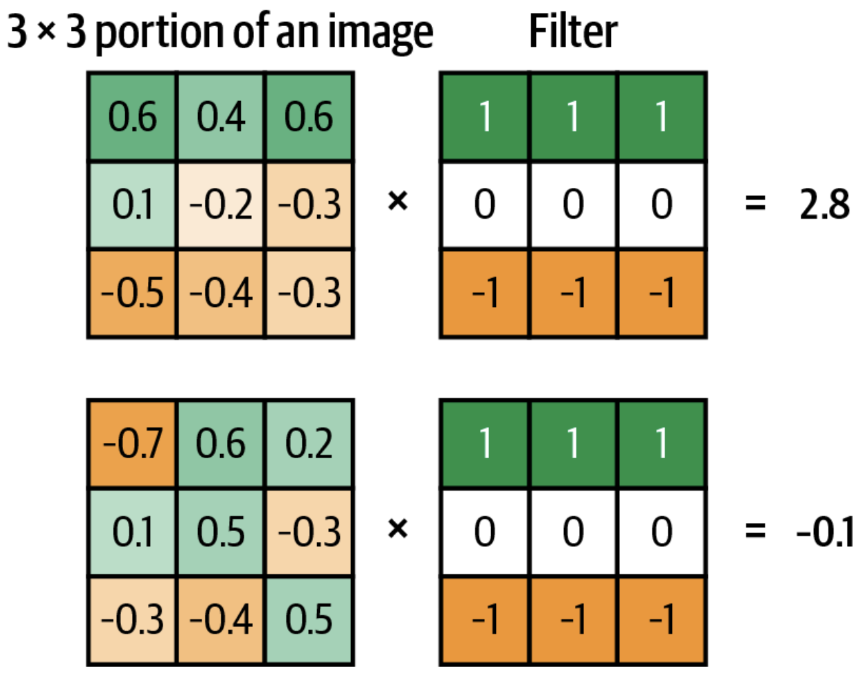
The convolution of the first image and the filter is 0.6*1 + 0.4*1 + 0.6*1 + 0.1*0 + (-0.2)*0 + (-0.3)*0 + (-0.5)*(-1) + (-0.4)*(-1) + (-0.3)*(-1) = 2.8.
The convolution of the second image and the filter is (-0.7)*1 + 0.6*1 + 0.2*1 + 0.1*0 + 0.5*0 + (-0.3)*0 + (-0.3)*(-1) + (-0.4)*(-1) + 0.5*(-1) = -0.1.
A positive convolution value indicates a better match between the filter and the image, while a negative value indicates a mismatch. In the above example, the convolution value of the first image and the filter is 2.8, indicating a match; the convolution value of the second image and the filter is -0.1, indicating a mismatch.
Filter
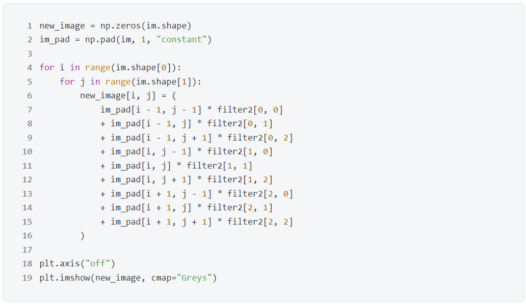
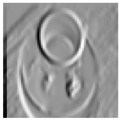
The purpose of a filter is to filter, which is equivalent to extracting and retaining certain information. The following code creates two 3*3 filters. Filter 1 can extract horizontal lines from the image, and filter 2 can extract vertical lines from the image. Note that here 1 represents black, 0 represents gray, and -1 represents white.
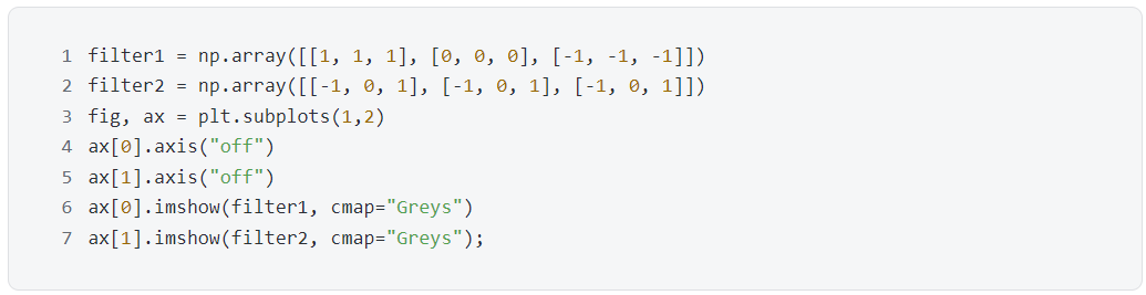

Now let's see how to use these two filters to extract information. The original image is shown below:
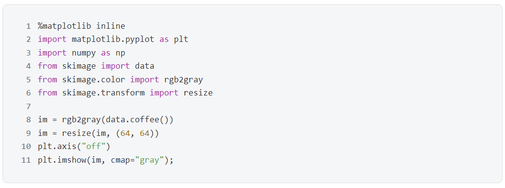
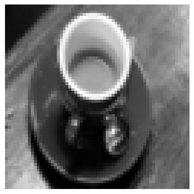
It is not difficult to find that filter 1 does extract the horizontal edge information from the image, such as the upper and lower edges of the cup.
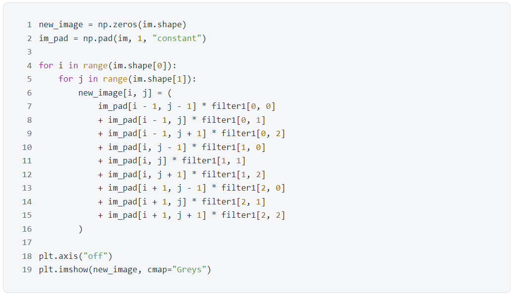
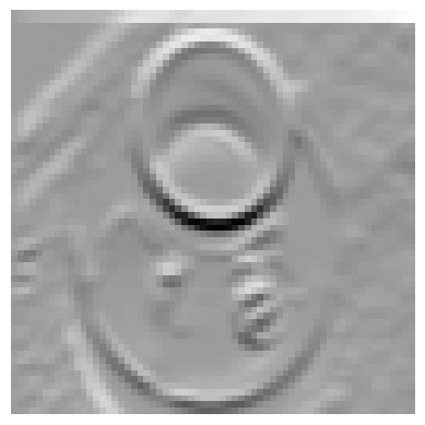
It is not difficult to find that filter 2 does extract the vertical edge information from the image, such as the left and right edges of the cup.
With the addition of filters, we can create a convolutional layer. The convolutional layer is essentially a set of filters, with 2 filters in the example below. The elements in the filters are called weights, which are learned through training the CNN.
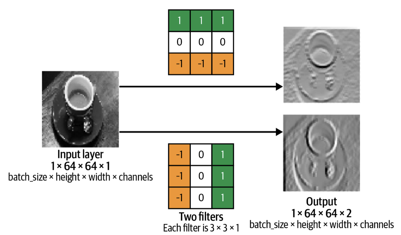
In Keras, we use layers.Con v 2 D() to create a convolutional layer. In this case, the grayscale image is 64* 64* 1 (with only 1 channel), and there are 2 filters (the filters parameter is set to 2), with filter size 3* 3 (the kernel_size parameter is set to ( 3, 3)).
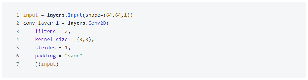
What are the parameters strides and padding?
Stride
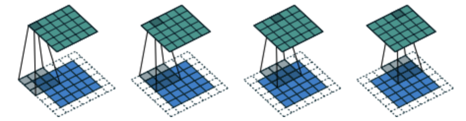
The stride is the number of pixels the filter moves when traversing the image. The default value is 1, meaning the filter moves one pixel at a time. When the stride is 2, it can be imagined that the size of the output image is only half of the input image size.
Padding
As the name suggests, padding refers to adding elements around the image. When padding = "same" and paired with strides = 1, the output image size can be ensured to be the same as the input image size. In the input image below (size 5* 5, shown in blue), after padding, the image size becomes 7* 7 (with white background), and the filter size is 3* 3 (shown in gray). The output image size remains 5* 5 (shown in green).
After understanding the components of a convolutional layer, we can concatenate convolutional layers just like how we concatenate dense layers in the previous section.
3.2 Concatenate Convolutional Layers
Let's take a look at some code:
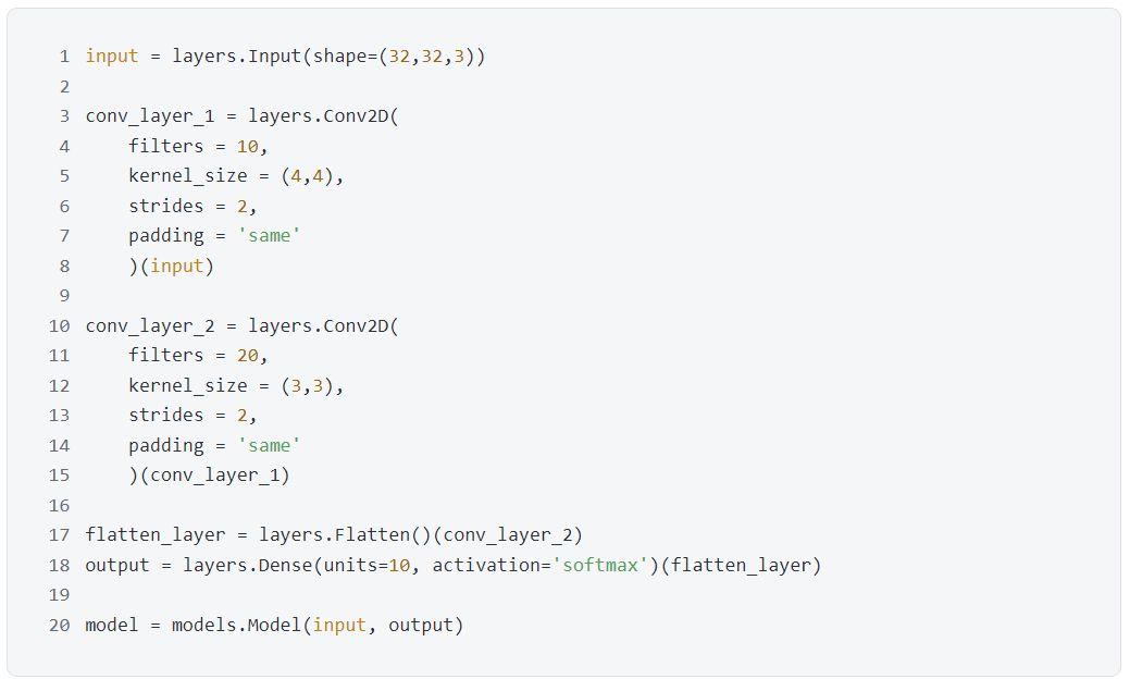
The above code corresponds to the appearance of the following image.
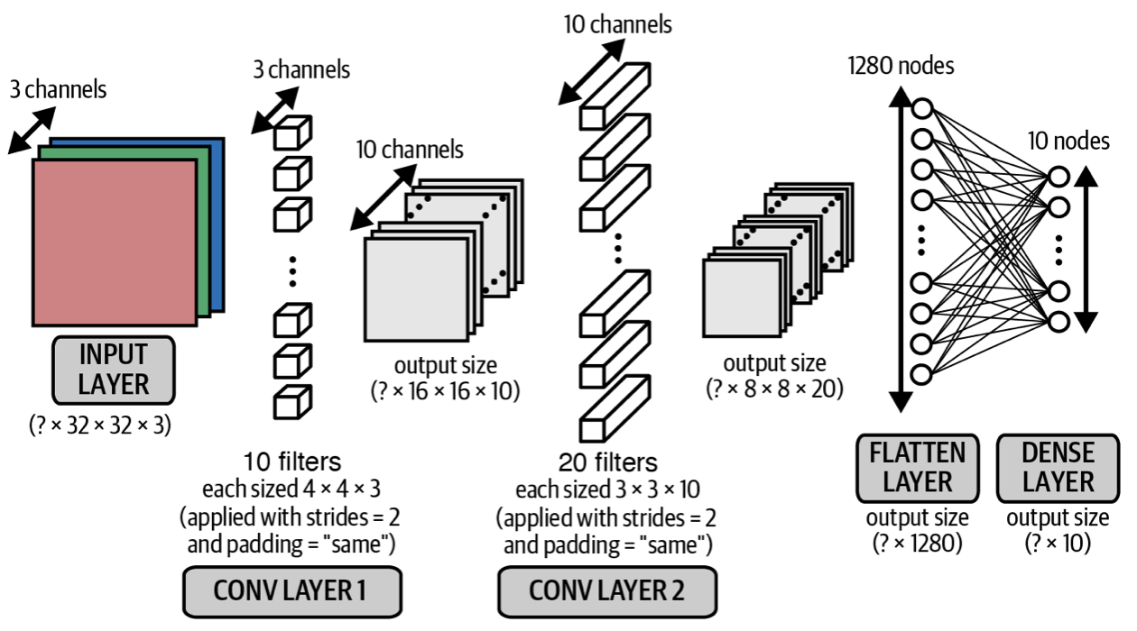
The size of each convolutional layer output above is dazzling. If we use n I to represent the size of the input image, f to represent the size of the filter, s to represent the stride, and p to represent the padding layer, then we have the following relationships:
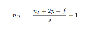
Use this formula to verify the width and height of the output of the first and second convolutional layers:
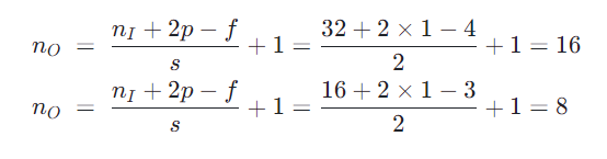
The most important thing is that the number of output channels of a convolutional layer is equal to the number of filters (the 'filters' parameter in the code). One intuitive understanding is that each filter parallelly scans the image and performs convolution, so the final output must have a dimension size equal to the number of filters.
Check the model.

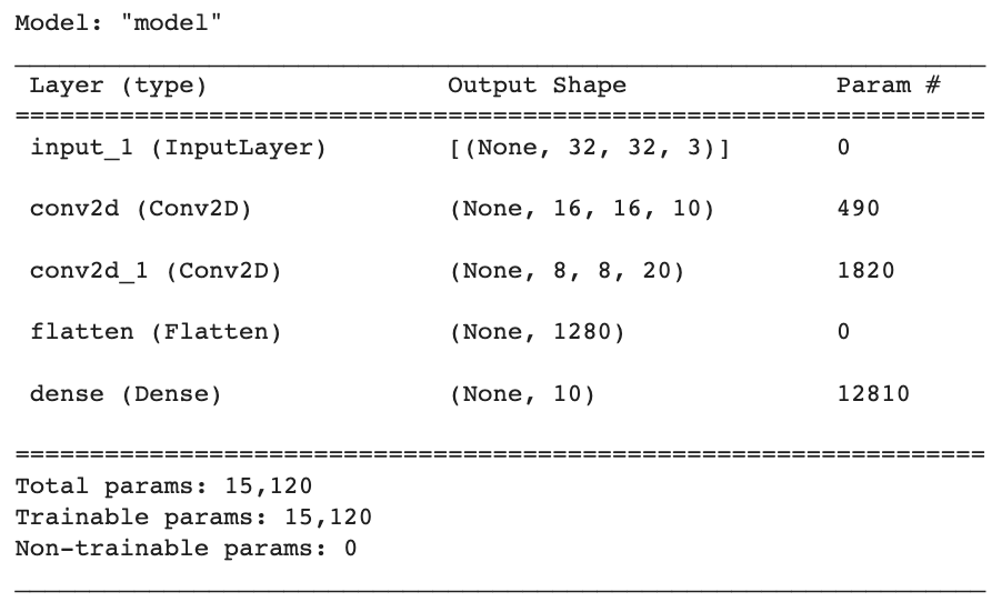
The model is automatically named "model", followed by a table describing the name type (layer (type)), output shape (Output Shape), and number of parameters (Param #) for each layer. Let's look at each layer:
The InputLayer is named input_1, with an output shape of [None, 32, 32, 3]. The last three elements correspond to the image width, height, and color channels, and the first None represents the number of samples in a batch. For code simplicity, this number of samples is usually not explicitly written during modeling.
The first Conv2D layer is named conv2d, with an output shape of [None, 16, 16, 10]. The parameters are 490 = (4*4*3 + 1) * 10. Remember to include the bias unit, and 4*4 is the size of the filters, and 3 is the number of input color channels. So we need 4*4*3 weights to describe each filter, totaling 10 filters.
The second Conv2D layer is named conv2d_1, with an output shape of [None, 8, 8, 20]. The parameters are 1,820 = (3*3*10 + 1) * 20. Similarly, consider the bias unit, and 3*3 is the size of the filters, and 10 is the number of input color channels. So we need 3*3*10 weights to describe this filter, totaling 20 filters.
The Flatten layer is named flatten, and the number 1,280 represents the flattened count of 8*8*20. The number of parameters is 0 because flattening reshapes the array without requiring any parameters.
The last Dense layer is named dense, with an output shape of 10. The parameters are 12,810 = (1280 + 1) * 10, considering the bias unit as well.
The bottom also lists the total number of parameters (Total params) 15,120, the number of trainable parameters (Trainable params) 15,120, and the number of non-trainable parameters (Non-trainable params) 0.
At this point, a CNN has been built. We can further improve the performance of the CNN by adding two techniques: batch normalization and dropout.
3.3 Batch Normalization
During training of the CNN, it is crucial to ensure that the weights stay within a certain range to avoid the problem of exploding gradients. Batch normalization can solve this problem by calculating the mean and standard deviation of the data in each layer per mini-batch, and then subtracting the mean and dividing by the standard deviation for each data point. To "restore" the data, we need to "learn" two parameters: the scaling parameter γ and the shifting parameter β.
The algorithm for batch normalization is as follows:
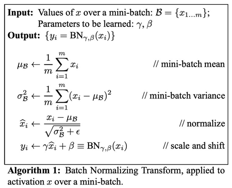
In Keras, you can use BatchNormalization() to implement the batch normalization layer. The batch normalization layer is usually placed after dense layers or convolutional layers.

The parameter "momentum" in the function is used to calculate the moving average and moving standard deviation. This is useful for prediction because during prediction, we usually have only one data point, so it is not possible to calculate the mean and standard deviation. In this case, we can only use the moving average and moving standard deviation calculated during training.
3.4 Dropout
Inspiration for random deactivation comes from exams. Typically, students would study past exam papers to learn the key points. Some students rely on memorization to solve problems, which can lead to poor performance in actual exams because they don't truly understand the key points. Good students use past papers to understand common knowledge points, allowing them to correctly answer new questions.
Similarly, to prevent neural networks from "memorizing" information, we can randomly deactivate certain neurons, setting their output to 0, as shown in the diagram below:
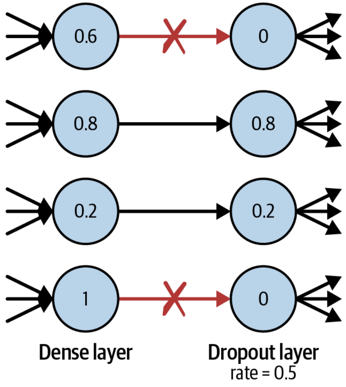
During the prediction process, neurons are not deactivated, so the complete neural network is used for prediction.
In Keras, the Dropout() function is used to implement dropout layers. Dropout layers are typically placed after dense layers.

The parameter "rate" in the function is used to set the dropout rate of neurons. In this example, 25% of the neurons are deactivated.
3.5 Complete Model
Now we can improve the previous CNN model by adding batch normalization layers and dropout layers.
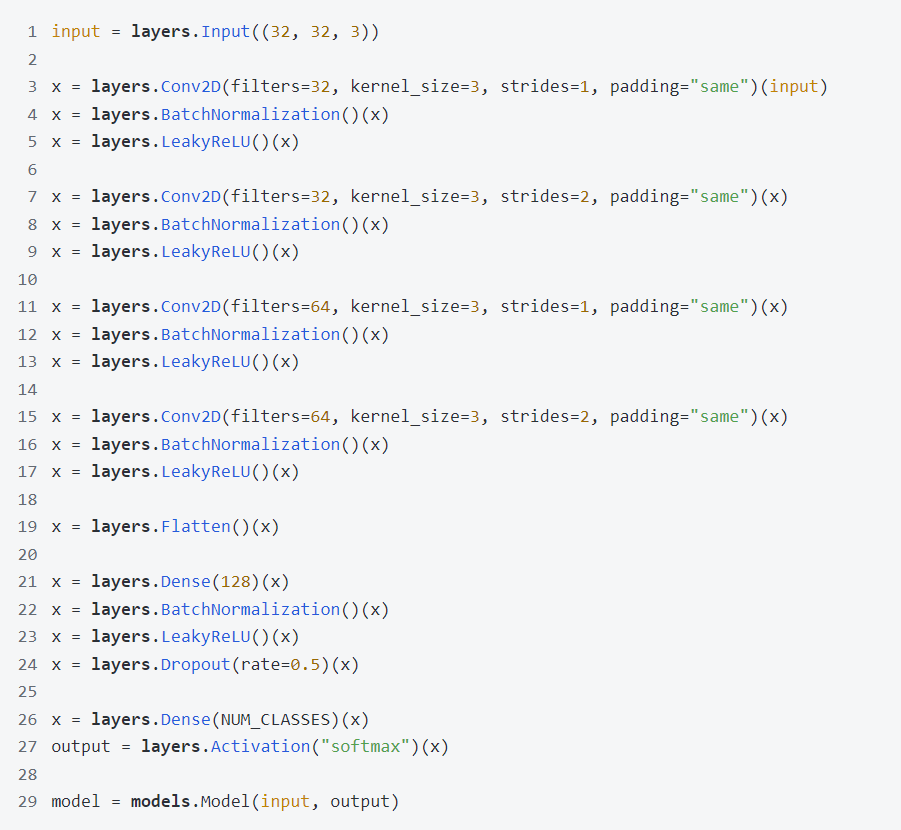
The code above should be easy to understand. This CNN has four convolutional layers, each followed by a batch normalization layer and a LeakyReLU layer. Note that in Keras, everything can be treated as a layer, even activation functions can be implemented as layers. Then a flatten layer is used to flatten the data, followed by a dense layer, a batch normalization layer, a LeakyReLU layer, a dropout layer, and finally a dense layer with softmax activation to output probabilities.
Let's check this improved CNN model.

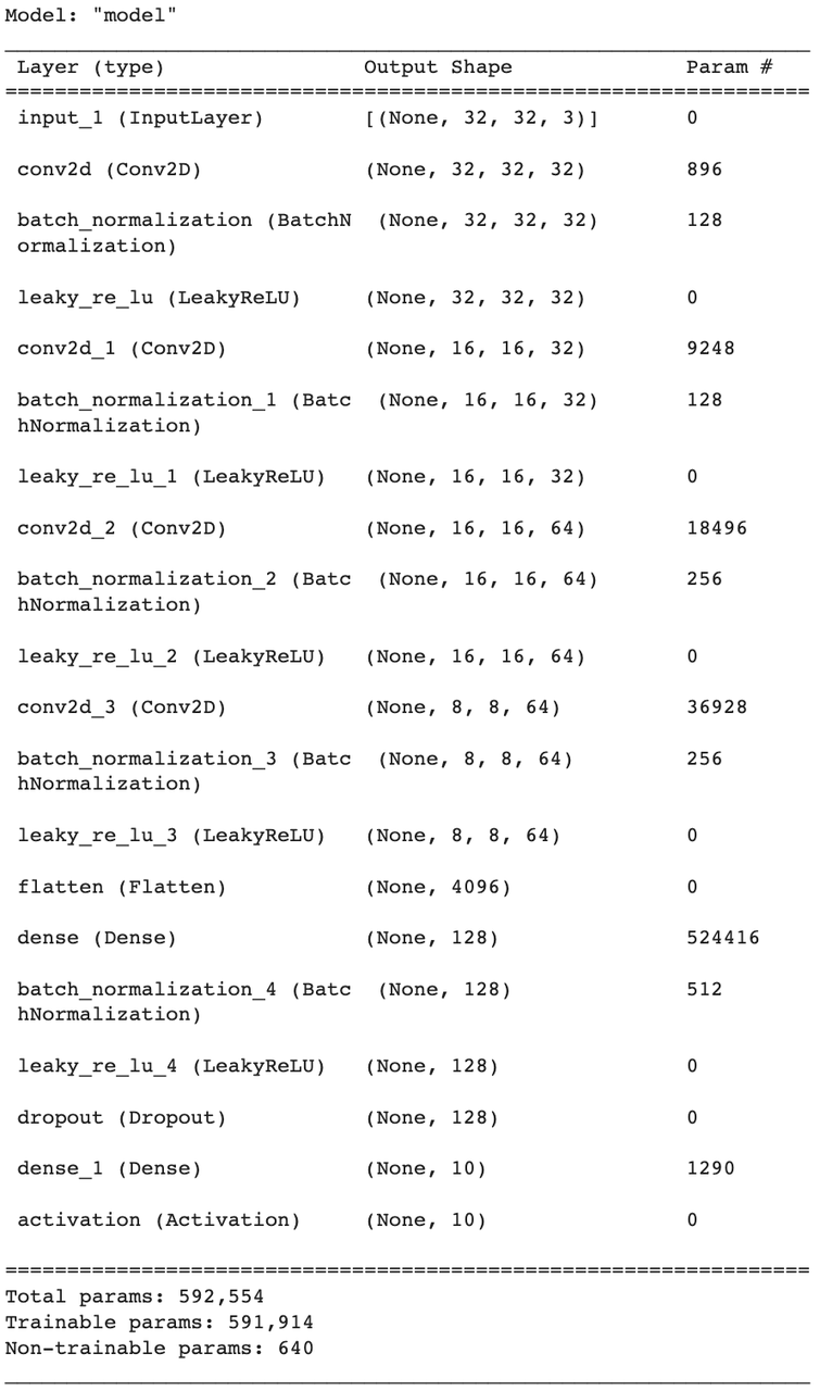
We found that the activation layer does not contain parameters, because it is just a transformation; the flatten layer and the dropout layer also do not contain parameters, which is also easy to understand; for the convolutional layer and the dense layer, the parameter count has been explained before; for the batch normalization layer, for each channel, we need to learn scaling parameter γ and shifting parameter β, as well as moving mean and moving standard deviation, so the number of parameters included is equal to the number of channels multiplied by 4.
In CNN, there are 5 batch normalization layers, and for each layer, the moving mean and moving standard deviation only need to be calculated without training, so the number of non-trainable parameters is 32 * 2 + 32 * 2 + 64 * 2 + 64 * 2 + 128 * 2 = 640.
3.6 Training Evaluation
Everything is ready, just waiting for training. This time we added a parameter called validation_data to monitor whether the model is overfitting during training. Overfitting occurs when the training error (loss) keeps decreasing while the validation error (val_loss) keeps increasing. From the figure below, this problem has not occurred yet.
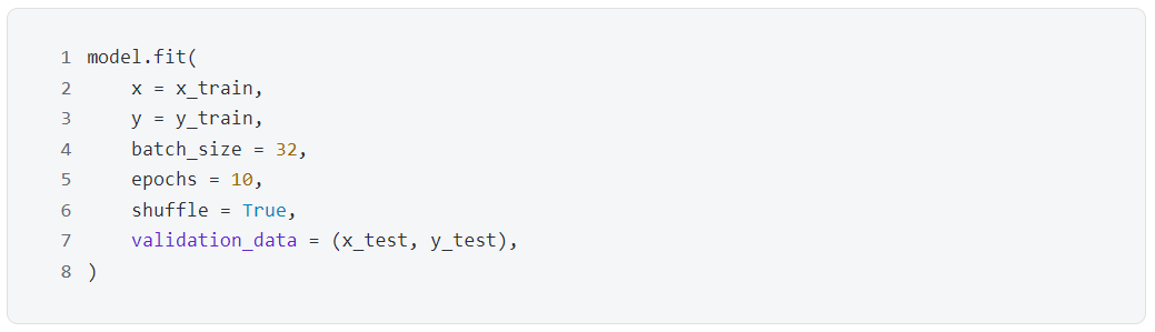
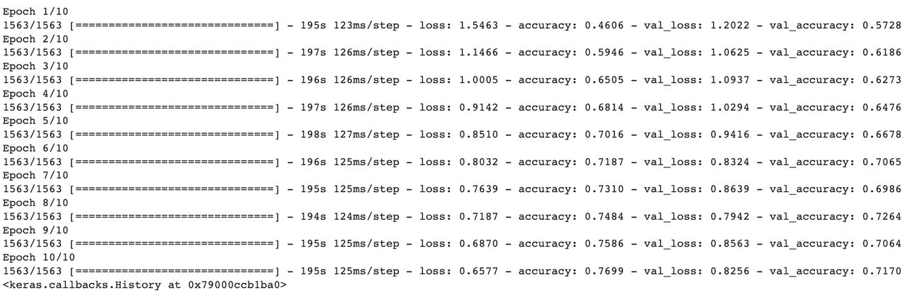


Compared to the previous feedforward neural network (FNN), the current model has improved the accuracy on the training set from 51.39% to 76.99%, and the accuracy on the test set from 49.52% to 71.70%. The model performance has greatly improved.
Interestingly, the CNN model has fewer parameters (592,554) compared to the FNN model (646,260), but it still achieves a significant improvement in performance. This improvement can be attributed to the inclusion of convolutional layers, batch normalization layers, and dropout layers in the CNN model architecture. Although CNN has fewer parameters than FNN, it has more layers. This is why deep neural networks have an advantage, as the intermediate layers capture high-level features that we are interested in.

From the 10 small images above, we can see that the model correctly predicts 6 images, achieving an accuracy of 60%. Although this is lower than the previously reported 71.70%, it is normal because these 10 images are sampled from a test set of 10,000 images. Therefore, it is reasonable to see the model correctly predicts images 6, 7, and 8.
Summary
This article introduces the core concepts of deep learning needed to build deep generative models. We start by building a feedforward neural network (FNN) using Keras and train it to predict the class of given images in the CIFAR-10 dataset. Then, we improve this architecture by introducing convolutional layers, batch normalization layers, and dropout layers to create a convolutional neural network (CNN).
Deep neural networks are highly flexible in design, and it is recommended to follow best practices. However, you can freely experiment with different layers and their ordering. Implementing them with Keras is as smooth as playing with LEGO bricks, and your neural network design is only limited by your imagination.
In the next article, we will use these modules to design a network that can generate images. The real show of generative AI is just beginning!
You can search for "SignalPlus" in the Plugin Store of ChatGPT 4.0 to get real-time encrypted information. If you want to receive our updates instantly, please follow our Twitter account @SignalPlus_Web 3 or join our WeChat group (add the assistant's WeChat: chillywzq), Telegram group, and Discord community to interact and communicate with more friends.
SignalPlus Official Website: https://www.signalplus.com


