
Learn how Python is applied to Coinbase in one article
The crypto space is a great way to experiment with different technologies. In this article, we'll cover the following:
How to load data from Coinbase Pro into Pandas dataframe?
How to convert and analyze historical cryptocurrency market data?
How to add Simple Moving Average (SMA), Exponential Moving Average (EMA), MACD, MACD Signal?
How to Visualize Cryptocurrency Market Data Using Plotly and Python?
This article only shows the most relevant Python code.

At the end of the article, we will be able to generate a cryptocurrency candle stick chart, including various performance indicators and market trends, like this:
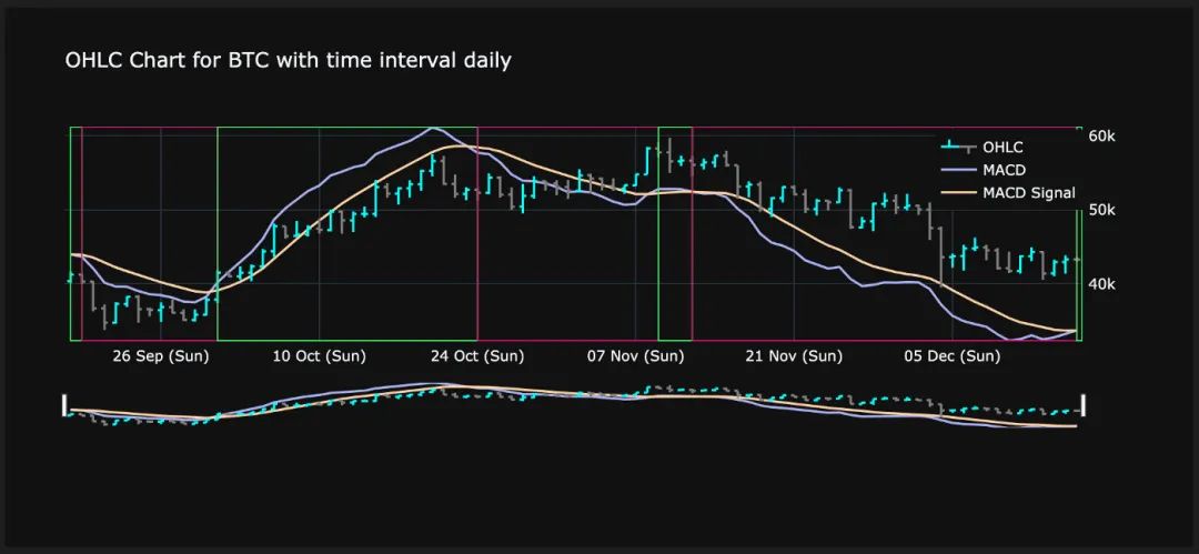
Final result - OHLC candlestick chart with market trend
Step 1: Connect to Coinbase Pro
With the help of the cbpro library, connecting to Coinbase Pro is a one-liner:
import cbpro
public_client = cbpro.PublicClient()
server_time = public_client.get_time()
# Server time does not comply to iso format, therefore slight modification of string needed
server_time_now = datetime.fromisoformat(server_time['iso'].replace('T', ' ', 1)[0:19])
print(server_time_now)
Launch public client to Coinbase Pro
We'll define a couple of constants because we want to limit the number of currencies we want to analyze. Let's also choose a base currency, such as USD or EUR, that we want to use to display the value of each currency.
FIAT_CURRENCIES = ['EUR','USD']
MY_BASE_CURRENCY = FIAT_CURRENCIES[0]
MY_CRYPTO_CURRENCIES = ["BTC","ETH","LTC","ALGO","SHIB","MANA"]
GRANULARITIES = ['daily','60min','15min','1min']
define constant
Step 2: Load statistics for the last 24 hours
Next, we'll review basic statistics for each cryptocurrency over the past 24 hours. We will also add a custom column "Performance" which will show the performance of the reporting period from start to end. The rest of the code takes care of number formatting.
currency_rows = []
for currency in MY_CRYPTO_CURRENCIES:
data = public_client.get_product_24hr_stats(currency+'-'+MY_BASE_CURRENCY)
currency_rows.append(data)
df_24hstats = pd.DataFrame(currency_rows, index = MY_CRYPTO_CURRENCIES)
df_24hstats['currency'] = df_24hstats.index
df_24hstats['open'] = df_24hstats['open'].astype(float)
df_24hstats['high'] = df_24hstats['high'].astype(float)
df_24hstats['low'] = df_24hstats['low'].astype(float)
df_24hstats['volume'] = df_24hstats['volume'].astype(float)
df_24hstats['last'] = df_24hstats['last'].astype(float)
df_24hstats['volume_30day'] = df_24hstats['volume_30day'].astype(float)
df_24hstats['performance'] = ((df_24hstats['last']-df_24hstats['open']) / df_24hstats['open']) * 100
df_24hstats_formatted = df_24hstats.copy()
df_24hstats_formatted['performance'] = df_24hstats_formatted['performance'].apply(lambda x: "{:.2f}%".format((x)))
df_24hstats_formatted['open'] = df_24hstats_formatted['open'].apply(lambda x: "{:,.2f}€".format((x)))
df_24hstats_formatted['high'] = df_24hstats_formatted['high'].apply(lambda x: "{:,.2f}€".format((x)))
df_24hstats_formatted['low'] = df_24hstats_formatted['low'].apply(lambda x: "{:,.2f}€".format((x)))
df_24hstats_formatted['last'] = df_24hstats_formatted['last'].apply(lambda x: "{:,.2f}€".format((x)))
df_24hstats_formatted.style.hide_columns(['volume','volume_30day'])
Load and format 24-hour market data for all cryptocurrencies from Coinbase Pro
image description
24-hour cryptocurrency data and performance
Step 3: Load historical data of different granularities
Next, we'll download historical market data using different time slice granularities. So we need to iterate over all currencies like step 2. Here is an example of how to retrieve daily data:
currency_history_rows = []
for currency in MY_CRYPTO_CURRENCIES:
start_date = (server_time_now - timedelta(days=90)).isoformat()
end_date = server_time_now.isoformat()
data = public_client.get_product_historic_rates(currency+'-'+MY_BASE_CURRENCY, start=start_date, end=end_date, granularity=86400)
[x.append(currency) for x in data]
[x.append('daily') for x in data]
currency_history_rows.extend(data)
df_history = pd.DataFrame(currency_history_rows)
df_history.columns = ['time','low','high','open','close','volume','currency','granularity']
df_history['date'] = pd.to_datetime(df_history['time'], unit='s')
In order to retrieve timeslice data, we need the following information:
The start date in ISO format of the desired time period
End date in ISO format for the desired time period
Granularity in seconds (in this case 86400 seconds, equal to 24 hours)
If you want to get hourly data for the past 300 hours, you can do the following:
start_date = (server_time_now - timedelta(hours=300)).isoformat()
end_date = server_time_now.isoformat()
data = public_client.get_product_historic_rates(currency+'-'+MY_BASE_CURRENCY, start=start_date, end=end_date, granularity=3600)
image description
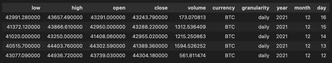
Cryptocurrency historical market data with daily time slice
Step Four: Add Metrics
Now comes the most challenging part. We want to add some custom investment metrics to our data. This will enhance the information we get from simple market data. We will add the following information:
SMA3 and SMA7 (simple moving average over the past 3 and 7 time slices): This is a price-based, lagging (or reactive) indicator that shows the average price of a security over a certain period of time. Moving averages remove "noise" when interpreting a chart. Noise is made up of price and volume fluctuations. The Simple Moving Average is an unweighted moving average. This means that each time period in the dataset has equal importance and is given equal weight.
EMA12 and EMA26 (exponential moving averages over the past 12 and 26 time slices): The EMA has much less lag than the SMA because it places more weight on recent prices. Therefore, it spins faster than the SMA. We could choose a different time slice, but 12 and 26 are commonly used durations and we will use them in our examples.
MACD (Moving Average Convergence/Divergence): A good indicator to determine the general trend of any security. It takes the difference between the short-term EMA and the long-term EMA. A positive MACD value is an indicator of a positive market trend. A negative MACD value is an indicator of a negative market trend.
MACD Signal: The MACD Signal line is the EMA on a specific time slice group of the MACD line. Typically, this value is set to 9 time slices.
MACD Histogram: This is the difference between the MACD Line and the MACD Signal Line. A bullish cross occurs when the MACD line crosses above the MACD signal line. A bearish cross occurs when the MACD line crosses below the MACD signal line. We'll see exactly what this means later, when we visualize the data.
Open-to-close performance: For each time slice, the difference between the close and open prices for a specific period is expressed as a percentage.
High-Low Span: The percentage deviation between the highest price and the lowest price within a period. This shows fluctuations within a time slice.
Absolute performance over the last 3 time periods: This indicator takes the performance of the last 3 time slices as an absolute value (measured in the base currency of choice we define in the constant).
Percentage of performance for the last 3 time periods: This indicator provides the performance of the last 3 time slices in the form of relative values (percentages).
Bull or Bear: If the MACD histogram is positive, write "bull"; if the MACD histogram is negative, write "bear".
Continuing market trend: To identify a transition from bull to bear and vice versa, this column is "True" if the trend from the previous time slice continues, and "False" if the trend has changed.
Thanks to Panda's powerful vector operations and built-in functions, we achieved this with just a few lines of code.
currency_history_rows_enhanced = []
for currency in MY_CRYPTO_CURRENCIES:
for granularity in GRANULARITIES:
df_history_currency = df_history.query('granularity == @granularity & currency == @currency').copy()
df_history_currency = df_history_currency.sort_values(['date'], ascending=True)
df_history_currency['SMA3'] = df_history_currency['close'].rolling(window=3).mean()
df_history_currency['SMA7'] = df_history_currency['close'].rolling(window=7).mean()
df_history_currency['EMA12'] = df_history_currency['close'].ewm(span=12, adjust=False).mean()
df_history_currency['EMA26'] = df_history_currency['close'].ewm(span=26, adjust=False).mean()
df_history_currency['MACD'] = df_history_currency['EMA12'] - df_history_currency['EMA26']
df_history_currency['MACD_signal'] = df_history_currency['MACD'].ewm(span=9, adjust=False).mean()
df_history_currency['macd_histogram'] = ((df_history_currency['MACD']-df_history_currency['MACD_signal']))
df_history_currency['open_to_close_perf'] = ((df_history_currency['close']-df_history_currency['open']) / df_history_currency['open'])
df_history_currency['high_low_span'] = ((df_history_currency['high']-df_history_currency['low']) / df_history_currency['high'])
df_history_currency['open_perf_last_3_period_abs'] = df_history_currency['open'].rolling(window=4).apply(lambda x: x.iloc[1] - x.iloc[0])
df_history_currency['open_perf_last_3_period_per'] = df_history_currency['open'].rolling(window=4).apply(lambda x: (x.iloc[1] - x.iloc[0])/x.iloc[0])
df_history_currency['bull_bear'] = np.where(df_history_currency['macd_histogram']< 0, 'Bear', 'Bull')
currency_history_rows_enhanced.append(df_history_currency)
df_history_enhanced = pd.concat(currency_history_rows_enhanced, ignore_index=True)
df_history_enhanced = df_history_enhanced.sort_values(['currency','granularity','date'], ascending=True)
df_history_enhanced['market_trend_continued'] = df_history_enhanced.bull_bear.eq(df_history_enhanced.bull_bear.shift()) & df_history_enhanced.currency.eq(df_history_enhanced.currency.shift()) & df_history_enhanced.granularity.eq(df_history_enhanced.granularity.shift())
Step Five: Use Information to Make Decisions
image description
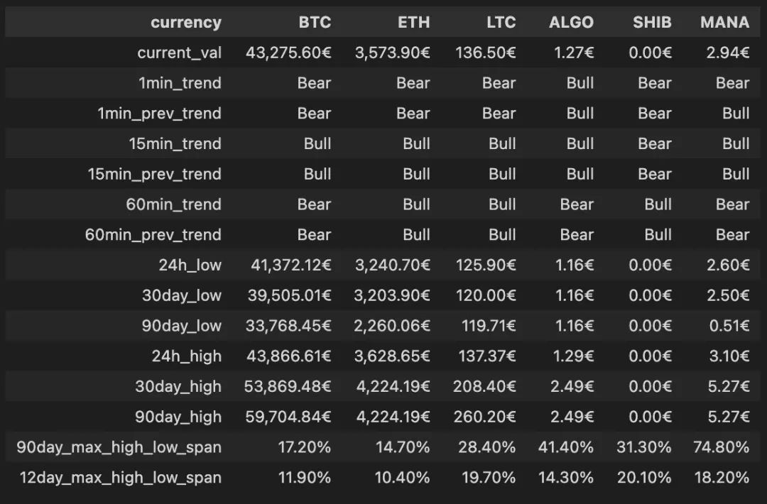
Performance of various cryptocurrencies over the past 90 days
Step Six: Visualize Crypto Market Data
In the final step, we want to visualize the underlying data built so far. For visualization, we will use the powerful Plotly library.
Before we can visualize the data, we need to create one more Pandas dataframe that will contain the information needed to plot the bearish (red) and bullish (green) boxes in the image below. Therefore, we need to construct a table that will give bull and bear market time periods, including start and end time periods. Thanks to Pandas, we can easily achieve this with the following code snippet:
market_trend_interval_rows = []
for currency in MY_CRYPTO_CURRENCIES:
for granularity in GRANULARITIES:
df_history_market_trend_intervals = df_history_enhanced.query('currency == @currency and market_trend_continued == False and granularity == @granularity').copy()
df_history_market_trend_intervals['next_period_date'] = df_history_market_trend_intervals.date.shift(-1)
df_history_market_trend_intervals['next_period_date'] = df_history_market_trend_intervals['next_period_date']
df_history_market_trend_intervals.next_period_date = df_history_market_trend_intervals.next_period_date.fillna(datetime.now())
df_history_market_trend_intervals['color'] = df_history_market_trend_intervals['bull_bear'].apply(lambda x: GREEN_COLOR if x == 'Bull' else RED_COLOR)
df_history_market_trend_intervals = df_history_market_trend_intervals[['currency','granularity','bull_bear','color','date','next_period_date']].rename(columns={"date": "start_date", "next_period_date": "finish_date"})
market_trend_interval_rows.append(df_history_market_trend_intervals)
df_history_market_trend_intervals = pd.concat(market_trend_interval_rows, ignore_index=True)
Powerful Pandas functions to transform our time slices
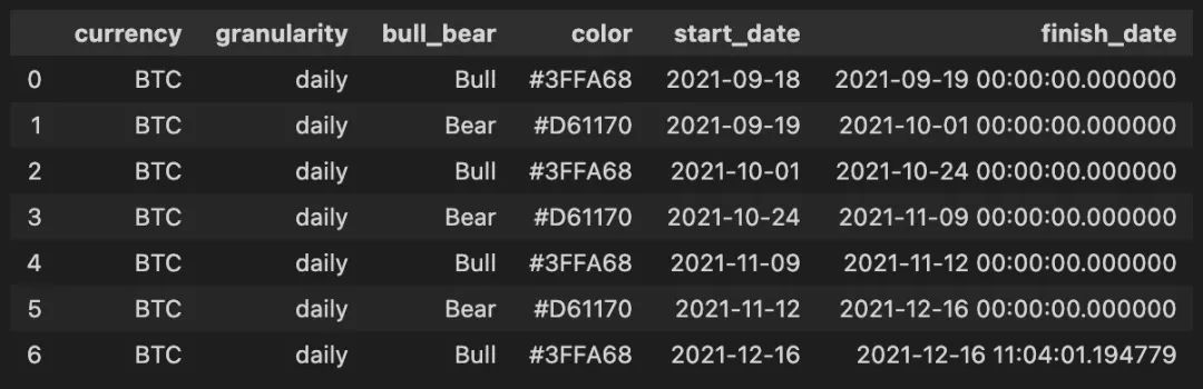
image description
Pandas dataframe with compressed bullish and bearish time periods
image description

Sophisticated cryptocurrency candlestick charts, including performance indicators and market trends
This chart uses two y-axes in Plotly. The y-axis on the right is used to draw candlesticks. The left y-axis is used to plot the MACD and the MACD signal line.
summary
summary
Original link


