
SignalPlus:自动编码器 (autoencoder)
原文作者:Steven Wang

前言
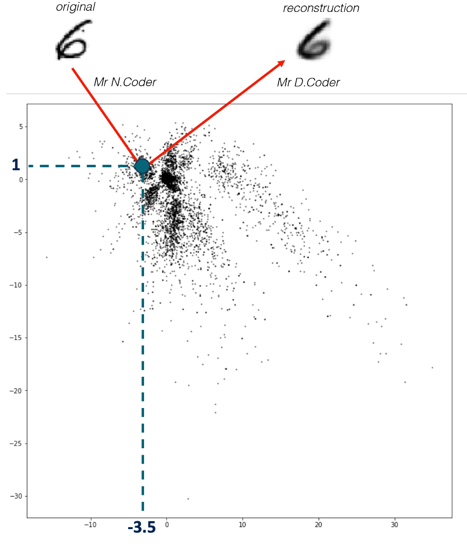
两兄弟 N.Coder 和 D.Coder 经营着一家艺术画廊。一周末,他们举办了一场特别奇怪的展览,因为它只有一面墙,没有实体艺术品。当他们收到一幅新画时,N.Coder 在墙上选择一个点作为标记来代表这幅画,然后扔掉原来的艺术品。当顾客要求观看这幅画时,D.Coder 尝试仅使用墙上相关标记的坐标来重新创作这件艺术品。
展墙如下图所示,每个黑点是 N.Coder 放置的一个标记,代表一幅画。在墙上坐标 [– 3.5, 1 ] 处的那幅原图 (original) 数字 6 的画 N.Coder 对其进行了重建 (reconstruction)。
下图展示了更多例子,顶行的数字是原图,中行的坐标是 N.Coder 将图挂在墙上的坐标,底行是 D.Coder 根据坐标重建的作品。
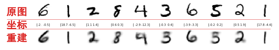
问题来了,N.Coder 如何决定每幅画在展墙上对应的坐标,而使得 D.Coder 仅用它就能重建原图的?原来是两兄弟在放置标记和重建作品的过程中,仔细监控售票处因顾客因重建质量不佳而要求退款而造成的收入损失,他们经过多年的“训练”逐渐“精通”标记放置和作品重建,而最大限度地减少这种收入损失。从上图对比原图和重建可以看出,两兄弟之间的磨合效果还不错。来参观艺术品的顾客很少抱怨 D.Coder 重新创作的画作与他们来参观的原始作品有很大的不同。
有一天,N.Coder 望着展墙,有了一个大胆的想法,对于那些墙上当前没有标记的部分,如果让 D.Coder 来重建能创作出什么样的作品?如果成功的话,那么他们就可以举办自己 100% 原创的画展了。想想就兴奋,于是 D.Coder 随机选取了之前没有标记的坐标 (红点) 来重建,结果如下图所示。
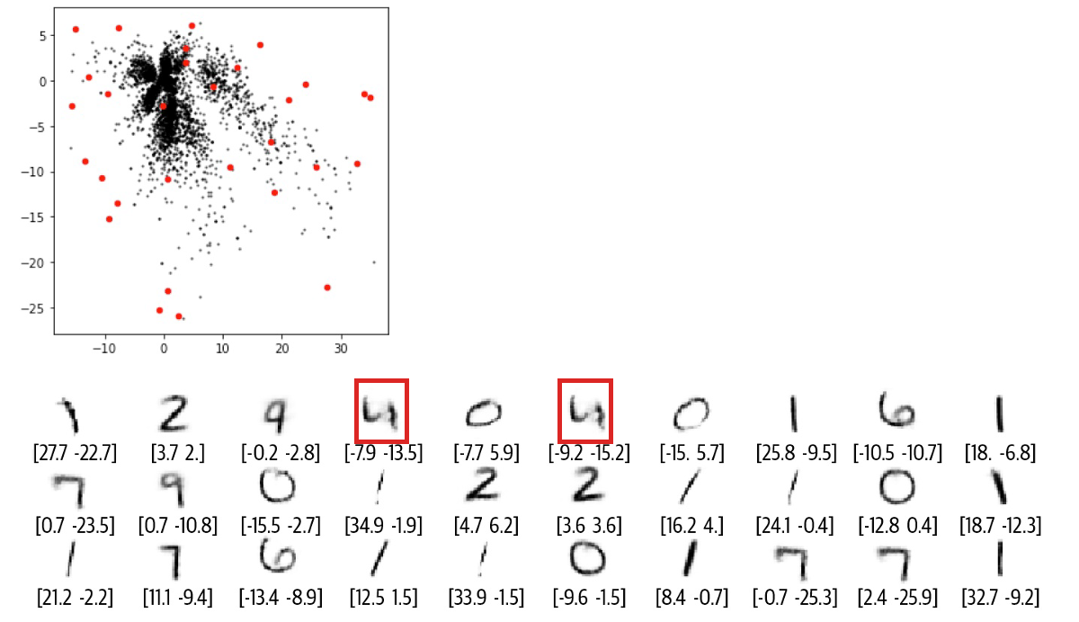
正如你所看到的,重建效果较差,有些图甚至都分辨不出是什么数字。那么到底出了什么问题,Coder 两兄弟该如何改进他们的方案呢?
1.自动编码器
前言的故事其实就是类比自动编码器 (autoencoder),D.Coder 音译为 encoder,即编码器,做的事情就是将图片转成坐标,而 N.Coder 音译为 decoder,即解码器,做的事情就是将坐标还原成图片。上节的两兄弟监控的收入损失其实就是模型训练时用的损失函数。
故事归故事,让我们看看自动编码器的严谨描述,它本质上就是一个神经网络,包含:
一个编码器 (encoder):用来把高维数据压缩成低维表征向量。
一个解码器 (decoder):用来将低维表征向量还原成高维数据。
该流程如下图所示,original input data 是高维图片数据,图片包含很多像素因此是高维的,而 representation vector 是低维表征向量,本例用的二维向量 [-2.0, -0.5 ] 是低维的。
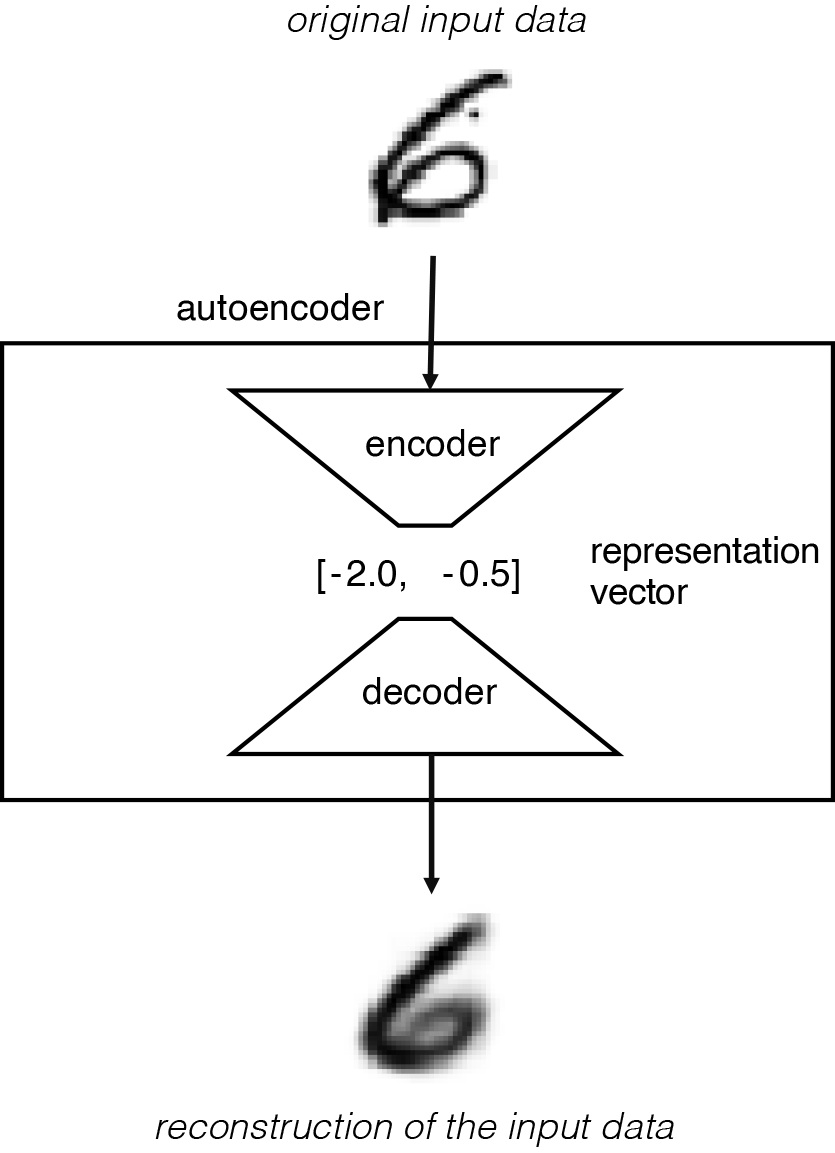
该网络经过训练,可以找到编码器和解码器的权重,最小化原始输入与输入通过编码器和解码器后的重建之间的损失。表征向量是将原始图像压缩到较低维的潜空间。 通过选择潜空间 (latent space) 中的任何点,我们应该能够通过将该点传递给解码器来生成新的图像,因为解码器已经学会了如何将潜空间中的点转换为可看的图像。
在前言描述中,N.Coder 和 D.Coder 使用表示二维潜空间 (墙壁) 内的向量对每个图像进行编码。之所以用二维是为了可视化潜空间,在实践中,潜空间通常高过两维,以便更自由地捕获图像中更大的细微差别。
2.模型解析
2.1 初次见面
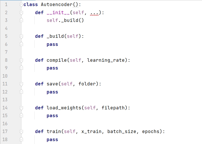
一般来说,最好用单独的文件来创建模型的类,比如下面的 Autoencoder class。这样其他项目可以灵活调用此类。下面代码首先展示了 Autoencoder 的框架,__init__() 是构造函数,通过调用 _build() 来创建模型,compile() 函数用于设定优化器,save() 函数用于保存模型,load_weights() 函数用于下次使用模型时加载权重,train() 函数用于训练模型。
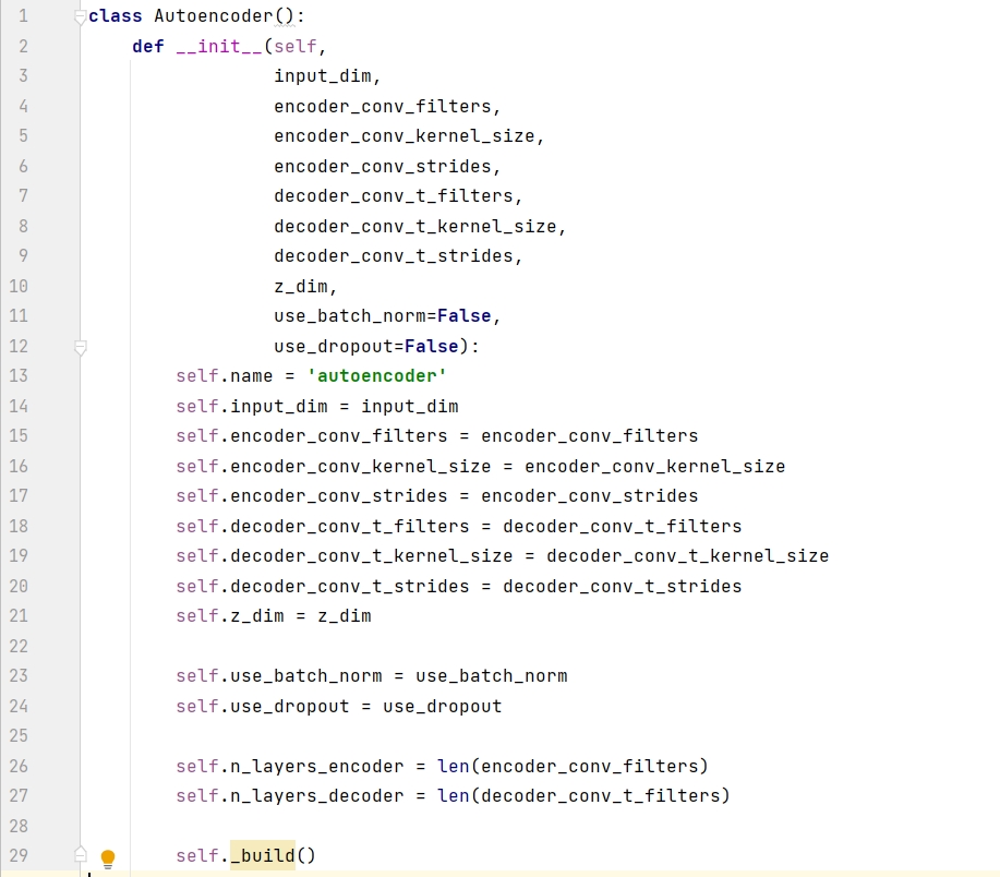
构建函数包含 8 个必需参数和 2 个默认参数,input_dim 是图片的维度,z_dim 是潜空间的维度,剩下的 6 个必需参数分别是编码器和解码器的滤波器个数 (filters)、滤波器大小 (kernel_size)、步长大小 (strides)。
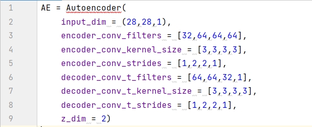
用构建函数创建自动编码器,命名为 AE。输入数据是黑白图片,其维度是 ( 28, 28, 1),潜空间用的 2D 平面,因此 z_dim = 2 。此外六个参数的值都是一个大小为 4 的列表,那么编码模型和解码模型都含有 4 层。
在 AutoEncoder 类里面定义 _build() 函数,构建编码器和解码器并将两者相连,代码框架如下 (后三小节会逐个分析):
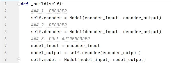
接下两小节我们来一一剖析自动编码器中的编码模型和解码模型。
2.2 编码模型
编码器的任务是将输入图片转换成潜空间的一个点,编码模型在 _build() 函数里面的具体实现如下:
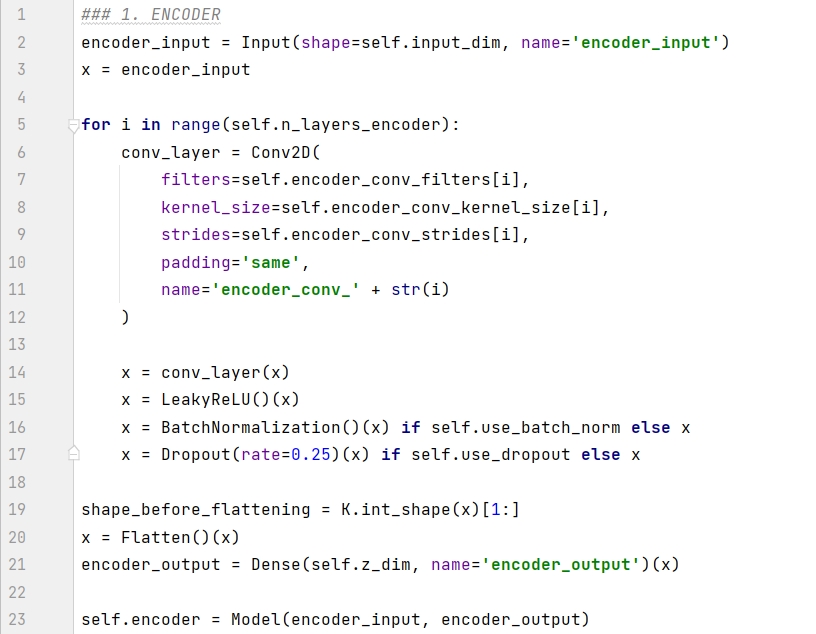
代码解释如下:
第 2-3 行将图片定义为 encoder 的输入。
第 5-17 行按顺序将卷积层堆起来。
第 19 行记录 x 的形状,K.int_shape 的返回是一个元组 (None, 7, 7, 64),第 0 个元素是样本大小,用 [ 1:] 返回除样本大小的数据形状 ( 7, 7, 64)。
第 20 行将最后的卷积层打平成为一个 1D 向量。
第 21 行的稠密层将该向量转成另一个大小为 z_dim 的 1D 向量。
第 22 行构建 encoder 模型,分别在 Model() 函数确定入参 encoder_input 和 encoder_output。
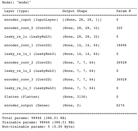
用 summary() 函数打印出编码模型的信息,用来描述每层的名称类型 (layer (type))、输出形状 (Output Shape) 和参数个数 (Param #)。

2.3 解码模型
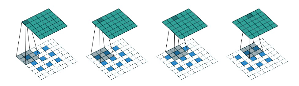
解码器是编码器的镜像,只不过不是使用卷积层,而是使用卷积转置层 (convolutional transpose layers) 来构建。当步长设为 2 ,卷积层每次将图片的高和宽减半,而卷积转置层将图片的高和宽翻倍。具体操作见下图。
解码器在 _build() 函数里面的具体实现如下:
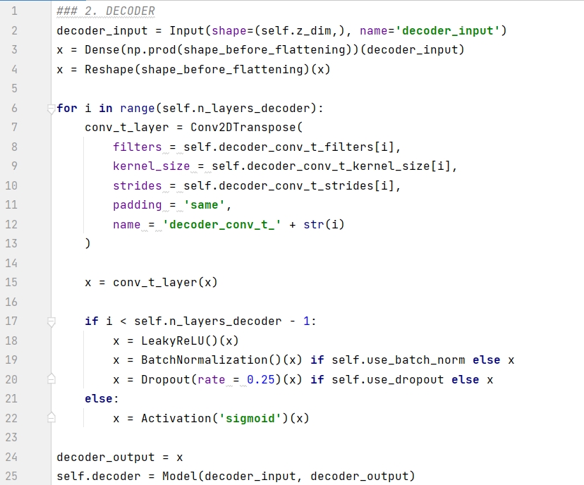
代码解释如下:
第 1 行将 encoder 的输出定义为 decoder 的输入。
第 2-3 行将 1D 向量重塑成形状为 ( 7, 7, 64) 的张量。
第 6-15 行按顺序将卷积转置层堆起来。
第 7-22 行:
如果是最后一层,用 sigmoid 函数转换,得到的结果在 0-1 之间当成像素
如果不是最后一层,用 leaky relu 函数转换,并加上批归一化 (batch normalization) 和随机失活 (dropout) 的处理。
第 24-25 行构建 decoder 模型,分别在 Model() 函数确定入参 decoder_input 和 decoder_output,前者是 encoder 的输出,即潜空间的点,而后者是重建的图片。
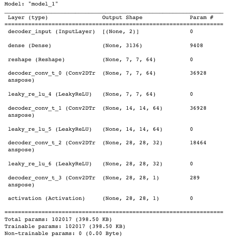
用 summary() 函数打印出解码模型的信息。

2.4 串连起来
为了能同时训练编码器和解码器,我们需要将两者连在一起,
代码解释如下:
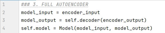
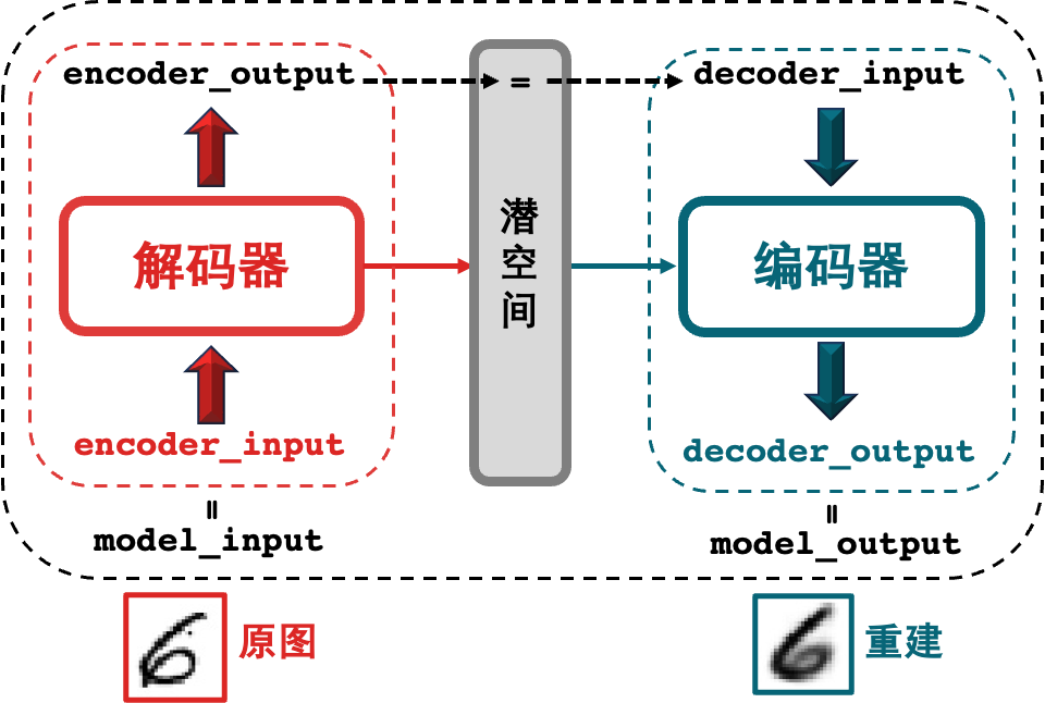
第 1 行将 encoder_input 作为整体模型的输入 model_input (中间产物 encoder_output 是编码器的输出)。
第 2 行将解码器的输出作为整体模型的输出 model_output (解码器的输入就是编码器的输出)。
第 3 行构建 autoencoder 模型,分别在 Model() 函数确定入参 model_input 和 model_output。
一图胜千言。
2.5 训练模型
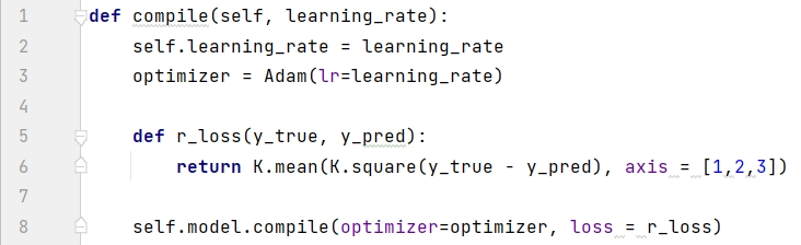
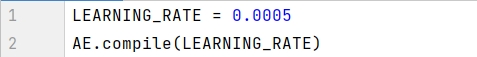
构建好模型之后,只需要定义损失函数和编译优化器。损失函数通常选择均方误差 (RMSE)。编译 complie() 函数的实现如下,用的是 Adam 优化器,学习率设为 0.0005 :
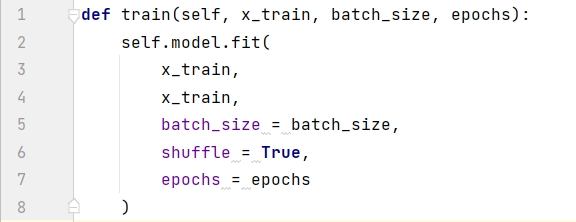
训练模型用 fit() 函数,批大小设为 32 ,epoch 设为 200 ,代码如下:

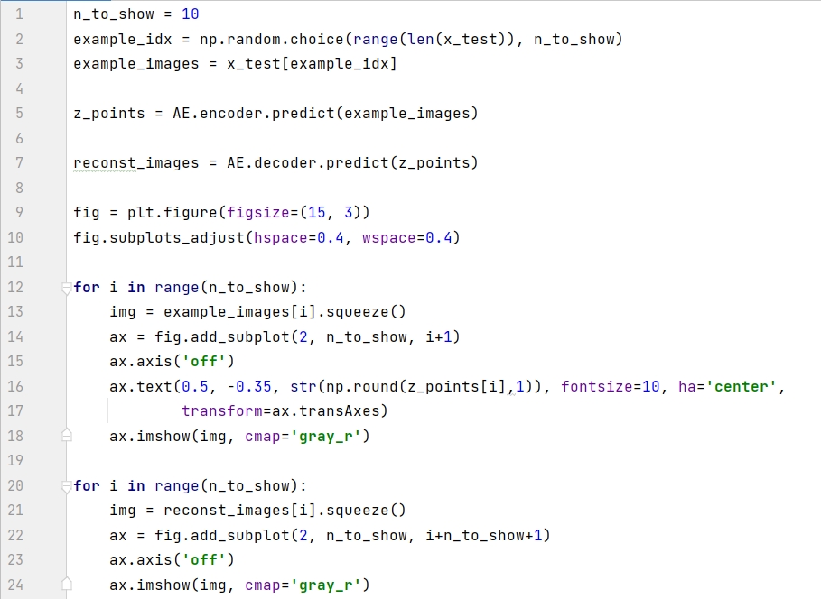
在测试集上随机选 10 个看看效果:
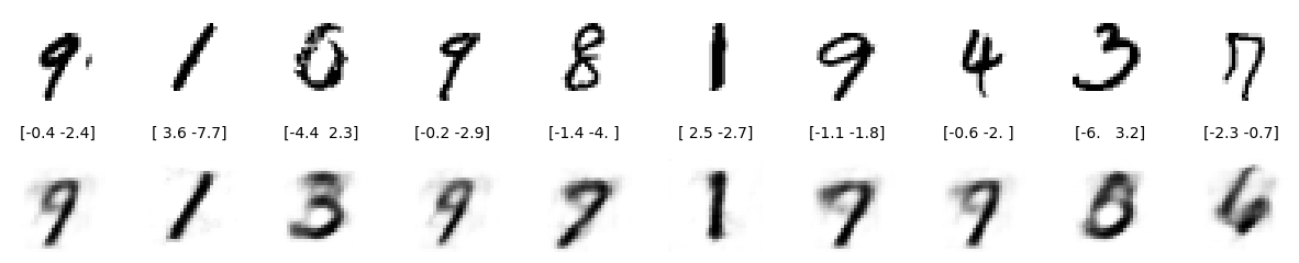
10 张图中只有 4 张重建效果还行。
3.三大缺陷
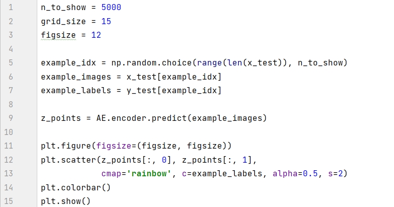
模型训练之后,我们可以可视化图片在潜空间的情况。通过模型中的 encoder 在测试集生成坐标在 2D 散点图中显示。
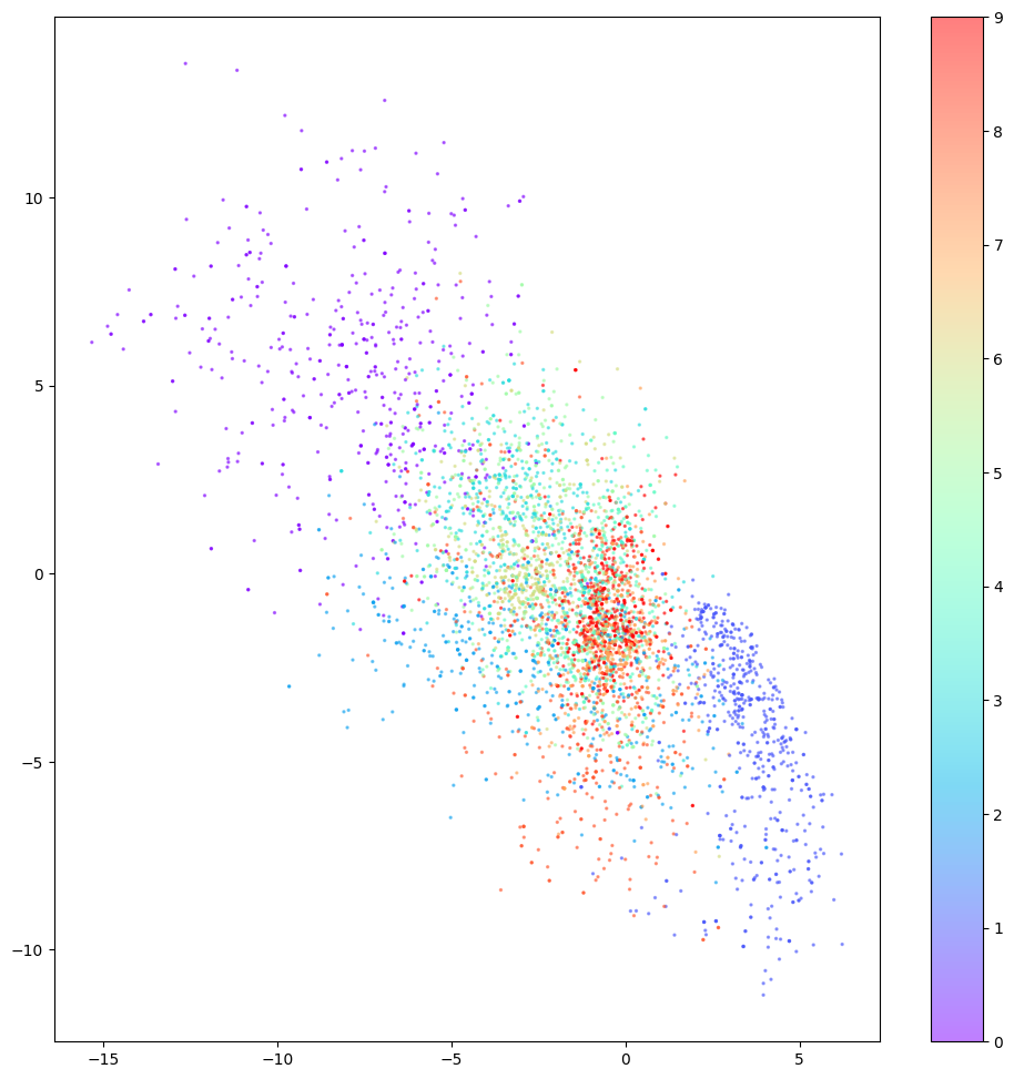
图中有三个现象值得注意:
有些数字的占地区域很小,比如红色的 9 ,有些数字的占地区域很大,比如紫色的 0 。
图中的点对于 ( 0, 0) 不对称,比如 x 轴上负值的点比正值的点会多很多,有些点甚至到了 x =-15 处。
颜色之间有很大的间隙,其中包含很少的点,如上图左上角。
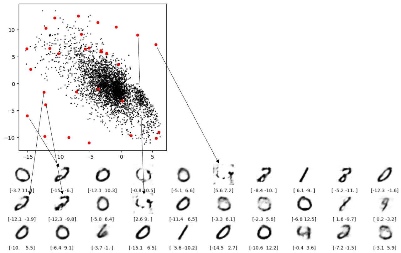
上述三大缺陷使我们从潜空间中采样非常困难:
对于缺陷 1 , 由于数字 9 比 0 的占地区域大,那么我们更容易采样到 9 。
对于缺陷 2 ,从技术上讲,我们可以采样平面上任何点。但每个数字的分布是不确定的,如果分布不是对称的话,那么随机采样的会很难操作。
对于缺陷 3 ,从下图可看出从潜空间中的空白处有的根本重构不出像样的数字。
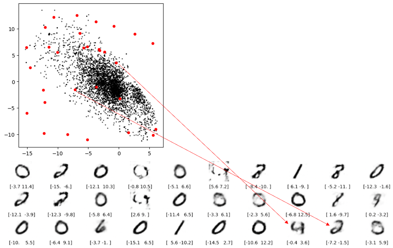
缺陷 3 空白出重构不出数字还好理解,但下图两条红线表示的重构就让人担忧了。这两个点都不在空白处,但是还是无法解码成像样的数字。根本原因就是自动编码器并没有强制确保生成的潜空间是连续的,例如,即便 ( 2,-2) 能够生成令人满意的数字 4 ,但该模型没有一个机制来确保点 ( 2.1, – 2.1) 也能产生令人满意的数字 4 。
总结
自动编码器只需要特征不需要标签,是一种无监督学习的模型,用于重建数据。该模型是一个生成模型,但从上节提到的三大缺陷,该生成模型对于低维黑白数字的效果都不好,那么对于高维彩色人脸的效果会更差。
这个自编码器框架是好的,那么我们应该如何解决这三个缺陷能生成一个强大的自动编码器。这个就是下篇的内容,变分自动编码器 (Variational AutoEncoder, VAE)。
您可在 ChatGPT 4.0 的 Plugin Store 搜索 SignalPlus,获取实时加密资讯。如果想即时收到我们的更新,欢迎关注我们的推特账号@SignalPlus_Web 3 ,或者加入我们的微信群(添加小助手微信:SignalPlus 123)、Telegram 群以及 Discord 社群,和更多朋友一起交流互动。
SignalPlus Official Website:https://www.signalplus.com


